
Chapter 8
Using Everyday Functions: Math, Date and Time, and Text Functions
Excel offers many functions for dealing with basic math, dates and times, and text. This chapter describes the functions that you can access with the Formulas tab using the Text icon, the Date & Time icon, and the Math portion of the Math & Trig icon.
Math Functions
Table 8.1 provides an alphabetical list of the math functions in Excel 2019. Detailed examples of these functions are provided later in this chapter.
Table 8.1 Alphabetical List of Math Functions
Function |
Description |
|---|---|
ABS(number) |
Returns the absolute value of a number. The absolute value of a number is the number without its sign. |
AGGREGATE(function, options, array, [k]) |
Performs one of 17 functions with the capability to ignore error values, other subtotals, or rows hidden by a filter. |
ARABIC(text) |
Converts a Roman numeral to Arabic. |
AVERAGEIF(range, criteria, [average_range]) |
Finds average (arithmetic mean) for the cells specified by a given condition or criteria. |
AVERAGEIFS(average_range, criteria_range1, criteria1, [criteria_range2, criteria2 …]) |
Returns the average value among cells specified by a given set of conditions or criteria. |
CEILING(number, significance) |
Returns the number rounded up, away from zero, to the nearest multiple of significance. For example, if you want to avoid using pennies in your prices and your product is priced at $4.42, you can use the formula =CEILING(4.42,0.05) to round the price up to the nearest nickel. Note that Excel calculates =CEILING(-2.1,-1) as –3, which is different from the ISO standard. See CEILING.MATH for an alternative. |
CEILING MATH(number, [significance],[mode]) |
Rounds a number up to the nearest multiple of significance. (Before Excel 2013, this function was named CEILING.PRECISE.) Provides compatibility with the ISO standard for computing the ceiling of a negative number. |
COMBIN(number,number_ chosen) |
Returns the number of combinations for a given number of items. You use COMBIN to determine the total possible number of groups for a given number of items. |
COMBINA(number,number_chosen) |
Returns the number of combinations with repetitions for a given number of items. |
COUNTIF(range,criteria) |
Counts the number of cells within a range that meet the given criteria. |
COUNTIFS(criteria_range1, criteria1, [criteria_range2,criteria2]…) |
Counts the number of cells within a range that meet the given set of conditions or criteria. |
EVEN(number) |
Returns the number rounded up to the nearest even integer. You can use this function for processing items that come in twos. For example, suppose a packing crate accepts rows of one or two items. The crate is full when the number of items, rounded up to the nearest two, matches the crate’s capacity. |
EXP(number) |
Returns e raised to the power of a number. The constant e equals 2.718281828459045, the base of the natural logarithm. Note that Excel 2016 began returning a 16th digit of precision, potentially causing different answers than Excel 2013. |
FACT(number) |
Returns the factorial of a number. The factorial of a number is equal to 1×2×3×…×number. |
FACTDOUBLE(number) |
Returns the double factorial of a number. |
FLOOR(number, significance) |
Rounds the number toward zero, to the nearest multiple of significance. |
FLOOR.MATH(number, [significance],[mode]) |
Rounds the number down to the nearest multiple of significance. (Before Excel 2013, this function was known as FLOOR.PRECISE.) Differs from FLOOR when you have negative numbers. Whereas FLOOR(-1.2,-1) rounds toward zero to produce –1, the new FLOOR.MATH(-1.2) rounds to the lower number, which is –2. |
GCD(number1,number2,…) |
Returns the greatest common divisor of two or more integers. The greatest common divisor is the largest integer that divides each number without a remainder. |
INT(number) |
Rounds a number down to the nearest integer. |
LCM(number1,number2,…) |
Returns the least common multiple of integers. The least common multiple is the smallest positive integer that is a multiple of all integer arguments number1, number2, and so on. You use LCM to add fractions that have different denominators. |
MAXIFS(max_range, criteria_range1, criteria1, [criteria_range2, criteria2…]) |
Returns the maximum value among cells specified by a given set of conditions or criteria. |
MINIFS(min_range, criteria_range1, criteria1, [criteria_range2, criteria2…]) |
Returns the minimum value among cells specified by a given set of conditions or criteria. |
MOD(number,divisor) |
Returns the remainder after a number is divided by the divisor. The result has the same sign as the divisor. |
MROUND(number,multiple) |
Returns a number rounded to the desired multiple. |
MULTINOMIAL(number1, number2,...) |
Returns the ratio of the factorial of a sum of values to the product of factorials. |
ODD(number) |
Returns a number rounded up to the nearest odd integer. |
PI() |
Returns the number 3.14159265358979, the mathematical constant pi, accurate to 15 digits. |
POWER(number, power) |
Returns the result of a number raised to a power. |
PRODUCT(number1, number2,...) |
Multiplies all the numbers given as arguments and returns the product. |
QUOTIENT(numerator, denominator) |
Returns the integer portion of a division operation. You use this function when you want to discard the remainder of a division. |
RAND() |
Returns an evenly distributed random number greater than or equal to 0 and less than 1. A new random number is returned every time the worksheet is calculated. |
RANDARRAY([rows],[columns]) |
Returns an array of random numbers. Office 365 exclusive. |
RANDBETWEEN(bottom, top) |
Returns a random number between the numbers specified. A new random number is returned every time the worksheet is calculated. |
ROMAN(number, form) |
Converts an Arabic numeral to Roman, as text. |
ROUND(number, num_ digits) |
Rounds a number to a specified number of digits. |
ROUNDDOWN(number, num_digits) |
Rounds a number down, toward zero. |
ROUNDUP(number,num_ digits) |
Rounds a number up, away from zero. |
SEQUENCE(rows,[columns],[start],[step]) |
Returns a sequence of numbers. Office 365 exclusive. |
SIGN(number) |
Determines the sign of a number. Returns 1 if the number is positive, 0 if the number is 0, and –1 if the number is negative. |
SQRT(number) |
Returns a positive square root. |
SQRTPI(number) |
Returns the square root of (number × pi). |
SUBTOTAL(function_num, ref1,ref2,...) |
Returns a subtotal in a list or database. It is generally easier to create a list with subtotals by using the Subtotals command (from the Data menu). After the subtotal list is created, you can modify it by editing the SUBTOTAL function. |
SUM(number1,number2,...) |
Adds all the numbers in a range of cells. |
SUMIF(range,criteria,sum_range) |
Adds the cells specified by the given criteria. |
SUMIFS(sum_range, criteria_range1, criteria1, [criteria_range2, criteria2 …] |
Adds the cells specified by a given set of conditions or criteria. |
SUMPRODUCT(array1,array2, array3,...) |
Multiplies corresponding components in the given arrays and returns the sum of those products. |
TRUNC(number,num_digits) |
Truncates a number to an integer by removing the fractional part of the number. |
Date and Time Functions
Table 8.2 provides an alphabetical list of the date and time functions in Excel 2019. Detailed examples of these functions are provided later in this chapter.
Table 8.2 Alphabetical List of Date and Time Functions
Function |
Description |
|---|---|
DATE (year, month, day) |
Returns the serial number that represents a particular date. |
DATEDIF (start_date, end_date, unit) |
Calculates the number of days, months, or years between two dates. This function is provided for compatibility with Lotus 1-2-3. |
DATEVALUE (date_text) |
Returns the serial number of the date represented by date_text. You use DATEVALUE to convert a date represented by text to a serial number. |
DAY (serial_number) |
Returns the day of a date, represented by a serial number. The day is given as an integer ranging from 1 to 31. |
DAYS (end_date, start_date) |
Calculates the difference in days between two dates. Works even if one or both dates are stored as text instead of as a date. |
DAYS360 (start_date, end_date, method) |
Returns the number of days between two dates, based on a 360-day year (that is, twelve 30-day months), which is used in some accounting calculations. You use this function to help compute payments if your accounting system is based on twelve 30-day months. |
EDATE (start_date, months) |
Returns the serial number that represents the date that is the indicated number of months before or after a specified date (that is, the start_date). You use EDATE to calculate maturity dates or due dates that fall on the same day of the month as the date of issue. |
EOMONTH (start_date, months) |
Returns the serial number for the last day of the month that is the indicated number of months before or after start_date. You use EOMONTH to calculate maturity dates or due dates that fall on the last day of the month. |
HOUR (serial_number) |
Returns the hour of a time value. The hour is given as an integer, ranging from 0 (12:00 a.m.) to 23 (11:00 p.m.). |
ISOWEEKNUM (date) |
Returns the ISO week number of the given date. |
MINUTE (serial_number) |
Returns the minutes of a time value. The minutes are given as an integer, ranging from 0 to 59. |
MONTH (serial_number) |
Returns the month of a date represented by a serial number. The month is given as an integer, ranging from 1 (for January) to 12 (for December). |
NETWORKDAYS (start_date, end_date, holidays) |
Returns the number of whole working days between start_date and end_date. Working days exclude weekends and any dates identified in holidays. You use NETWORKDAYS to calculate employee benefits that accrue based on the number of days worked during a specific term. Weekdays are defined as Saturday and Sunday. To handle other calendars, see NETWORKDAYS.INTL. |
NETWORKDAYS.INTL (start_date, end_date, weekend, holidays) |
Returns the number of whole working days between the start date and the end date. Added in Excel 2010 to support calendars in which the weekend is a pair of days other than Saturday and Sunday. |
NOW () |
Returns the serial number of the current date and time. |
SECOND (serial_number) |
Returns the seconds of a time value. The seconds are given as an integer in the range 0 to 59. |
TIME (hour, minute, second) |
Returns the decimal number for a particular time. The decimal number returned by TIME is a value ranging from 0 to 0.99999999, representing the times from 0:00:00 (12:00:00 a.m.) to 23:59:59 (11:59:59 p.m.). |
TIMEVALUE (time_text) |
Returns the decimal number of the time represented by a text string. The decimal number is a value ranging from 0 to 0.99999999, representing the times from 0:00:00 (12:00:00 a.m.) to 23:59:59 (11:59:59 p.m.). |
TODAY () |
Returns the serial number of the current date. The serial number is the date/time code that Microsoft Excel uses for date and time calculations. |
WEEKDAY (serial_number, return_type) |
Returns the day of the week corresponding to a date. The day is given as an integer, ranging from 1 (for Sunday) to 7 (for Saturday), by default. |
WEEKNUM (serial_num, return_type) |
Returns a number that indicates where the week falls numerically within a year. See also ISOWEEKNUM. |
WORKDAY (start_date, days, holidays) |
Returns a number that represents a date that is the indicated number of working days before or after a date (the starting date). Working days exclude weekends and any dates identified as holidays. You use WORKDAY to exclude weekends and holidays when you calculate invoice due dates, expected delivery times, or the number of days of work performed. To view the number as a date, format the cell as a date. Weekends are defined as Saturday and Sunday. For alternative calendars, see WORKDAY.INTL. |
WORKDAY.INTL (start_date, days, weekend, holidays) |
Returns a number that represents a date that is the indicated number of working days before or after a starting date. Added to Excel 2010 to accommodate calendar systems where the weekend is a pair of days other than Saturday and Sunday. |
YEAR (serial_number) |
Returns the year corresponding to a date. The year is returned as an integer in the range 1900 through 9999. |
YEARFRAC (start_date, end_date, basis) |
Calculates the fraction of the year represented by the number of whole days between two dates (start_date and end_date). You use the YEARFRAC worksheet function to identify the proportion of a whole year’s benefits or obligations to assign to a specific term. |
Text Functions
Table 8.3 provides an alphabetical list of the text functions in Excel 2019. Detailed examples of these functions are provided later in this chapter.
Table 8.3 Alphabetical List of Text Functions
Function |
Description |
|---|---|
ASC (text) |
Changes full-width (double-byte) English letters or katakana within a character string to half-width (single-byte) characters. |
BAHTTEXT (number) |
Converts a number to Thai text and adds the suffix Baht. |
CHAR (number) |
Returns the character specified by number. You use CHAR to translate code page numbers you might get from files on other types of computers into characters. See also UNICHAR. |
CLEAN (text) |
Removes all nonprintable characters from text. You use CLEAN on text imported from other applications that contains characters that might not print with your operating system. For example, you can use CLEAN to remove some low-level computer code that frequently appears at the beginning and end of data files and cannot be printed. |
CODE (text) |
Returns a numeric code for the first character in a text string. The returned code corresponds to the character set used by your computer. See also UNICODE. |
CONCAT (Text1, [Text2…]) |
Concatenates a list or range of text strings. |
CONCATENATE (text1, text2,...) |
Joins several text strings into one text string. |
DOLLAR (number, decimals) |
Converts a number to text using currency format, with the decimals rounded to the specified place. The format used is $#,##0.00_);($#,##0.00). |
EXACT (text1, text2) |
Compares two text strings and returns TRUE if they are the same and FALSE otherwise. EXACT is case-sensitive but ignores formatting differences. You use EXACT to test text being entered into a document. |
FIND (find_text, within_text, start_num) |
Finds one text string (find_text) within another text string (within_text) and returns the number of the starting position of find_text, from the first character of within_text. You can also use SEARCH to find one text string within another, but unlike SEARCH, FIND is case sensitive and doesn’t allow wildcard characters. |
FINDB (find_text, within_text, start_num) |
Finds one text string (find_text) within another text string (within_text) and returns the number of the starting position of find_text, based on the number of bytes each character uses, from the first character of within_text. You use FINDB with double-byte characters. You can also use SEARCHB to find one text string within another. |
FIXED (number, decimals, no_commas) |
Rounds a number to the specified number of decimals, formats the number in decimal format using a period and commas, and returns the result as text. |
LEFT (text, num_chars) |
Returns the first character or characters in a text string, based on the number of characters specified. |
LEFTB (text, num_bytes) |
Returns the first character or characters in a text string, based on the number of bytes specified. You use LEFTB with double-byte characters. |
LEN (text) |
Returns the number of characters in a text string. |
LENB (text) |
Returns the number of bytes used to represent the characters in a text string. You use LENB with double-byte characters. |
LOWER (text) |
Converts all uppercase letters in a text string to lowercase. |
MID (text, start_num, num_chars) |
Returns a specific number of characters from a text string, starting at the position specified, based on the number of characters specified. |
MIDB (text, start_num, num_bytes) |
Returns a specific number of characters from a text string, starting at the position specified, based on the number of bytes specified. You use MIDB with double-byte characters. |
NUMBERVALUE (text, [decimal_separator], [group_separator]) |
Converts text to a number, allowing for different punctuation for thousands separators and decimal separators. |
PHONETIC (reference) |
Extracts the phonetic (furigana) characters from a text string. Furigana are a Japanese reading aid. They consist of smaller kana printed next to a kanji to indicate its pronunciation. |
PROPER (text) |
Capitalizes the first letter in a text string and any other letters in text that follow any character other than a letter. Converts all other letters to lowercase. |
REPLACE (old_text, start_num, num_chars, new_text) |
Replaces part of a text string, based on the number of characters specified, with a different text string. |
REPLACEB (old_text, start_num, num_bytes, new_text) |
Replaces part of a text string, based on the number of bytes specified, with a different text string. You use REPLACEB with double-byte characters. |
REPT (text, number_times) |
Repeats text a given number of times. You use REPT to fill a cell with some instances of a text string. |
RIGHT (text, num_chars) |
Returns the last character or characters in a text string, based on the number of characters specified. |
RIGHTB (text, num_bytes) |
Returns the last character or characters in a text string, based on the number of bytes specified. You use RIGHTB with double-byte characters. |
SEARCH (find_text, within_text, start_num) |
Returns the number of the character at another a specific character or text string is first found, beginning with start_num. You use SEARCH to determine the location of a character or text string within another text string so that you can use the MID or REPLACE function to change the text. |
SEARCHB (find_text, within_text, start_num) |
Finds one text string (find_text) within another text string (within_text) and returns the number of the starting position of find_text. The result is based on the number of bytes each character uses, beginning with start_num. You use SEARCHB with double-byte characters. You can also use FINDB to find one text string within another. |
SUBSTITUTE (text, old_text, new_text, instance_num) |
Substitutes new_text for old_text in a text string. You use SUBSTITUTE when you want to replace specific text in a text string; you use REPLACE when you want to replace any text that occurs in a specific location in a text string. |
T (value) |
Returns the text referred to by value. |
TEXT (value, format_text) |
Converts a value to text in a specific number format. |
TEXTJOIN (delimiter, ignore_empty, text1, [text2…]) |
Concatenates a list of range of text strings using a delimiter. |
TRIM (text) |
Removes all spaces from text except for single spaces between words. You use TRIM on text that you have received from another application that might have irregular spacing. |
UNICHAR (number) |
Returns the Unicode character references by the given number. |
UNICODE (text) |
Returns the number (code point) of the first character of the text. |
UPPER (text) |
Converts text to uppercase. |
VALUE (text) |
Converts a text string that represents a number to a number. |
Examples of Math Functions
The most common formula in Excel is a formula to add a column of numbers. In addition to SUM, Excel offers a variety of mathematical functions.
Using SUM to Add Numbers
The SUM function is by far the most commonly used function in Excel. This function can add numbers from one or more ranges of data.
Syntax:
=SUM(number1,number2,...)
The SUM function adds all the numbers in a range of cells. The arguments number1, number2,... are 1 to 255 arguments for which you want the total value or sum.
A typical use of this function is =SUM(B4:B12). It is also possible to use =SUM(1,2,3). In the latter example, you cannot specify more than 255 individual values. In the former example, you can specify up to 255 ranges, each of which can include thousands or millions of cells.
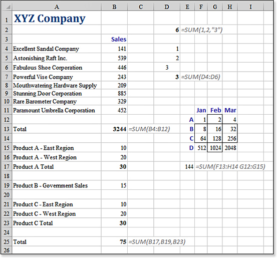
In Figure 8.1, cell B25 contains a formula to sum three individual cells: =SUM(B17,B19,B23).
SUM formulas.It is unlikely that you will need more than 255 arguments in this function, but if you do, you can group arguments in parentheses. For example, =SUM((A10,A12),(A14,A16)) would count as only two of the 255 allowed arguments.
If a text value that looks like a number is included in a range, the text value is not included in the result of the sum. Strangely enough, if you specify the text value directly as an argument in the function, Excel adds it to the result. For example, =SUM(1,2,"3") is 6, yet =SUM(D4:D6) in cell D7 of Figure 8.1 results in 3.
The comma is treated as a union operator. If you replace the comma with a space, Excel finds the cells that fall in the intersection of the selected ranges. In cell E17, the formula of =SUM(F13:H14 G12:G15) adds up the two cells that are in common between the two ranges.
If one cell in a referenced range contains an error, the result of the SUM function is an error. To add numbers while ignoring error cells, use the AGGREGATE function.
It is valid to create a spearing formula. This type of formula adds the identical cell from many worksheets. For example, =SUM(Jan:Dec!B20) adds cell B20 on all 12 sheets between Jan and Dec. If the sheet names contain spaces or other nonalphabetic characters, surround the sheet names with apostrophes: =SUM('Jan 2018:Dec 2018'!B20).
Using AGGREGATE to Ignore Error Cells or Filtered Rows
Added in Excel 2010, the AGGREGATE function lets you perform 17 functions on a range of data while selectively ignoring error cells or rows hidden by a filter.
Syntax:
=AGGREGATE(function_num, options, array, [k])
The options argument is the interesting feature of the function. You can choose to ignore any, all, or none of these categories:
Error values
Hidden rows
Other
SUBTOTALandAGGREGATEfunctions
The capability to ignore filtered rows and other AGGREGATE functions is similar to the SUBTOTAL function. The capability of AGGREGATE to ignore error values solves a common Excel problem. For most Excel functions, a single #N/A error cell in a range causes most functions to return an #N/A error. The options in AGGREGATE enable you to ignore any error cells in the range.
The options argument controls which values are ignored. This is a simple binary system, as follows:
To ignore other subtotals, add 0. To include subtotals, add 4.
To ignore hidden rows, add 1.
To ignore error values, add 2.
Thus, to ignore other subtotals, hidden rows, and error values, you specify
3 (0+1+2)as theoptionsargument.To ignore error values but include other
SUBTOTALvalues, you specify5 (1+4)as the argument.
This calculation works out as shown in Table 8.4.
Table 8.4 Arguments for the AGGREGATE Function
Option |
Meaning |
|---|---|
0 |
Ignore other subtotals |
1 |
Ignore hidden rows and subtotals |
2 |
Ignore error cells and subtotals |
3 |
Ignore all three |
4 |
Ignore nothing |
5 |
Ignore hidden rows |
6 |
Ignore error cells |
7 |
Ignore hidden rows and error cells |
In Figure 8.2, the #N/A error in cell F13 causes the SUM function in F18 to also return an #N/A. If you use a 2, 3, 5, or 7 as the second argument of AGGREGATE, you can easily sum all the other numbers as in cell F1. You can also use other function numbers to calculate MIN, MAX, COUNT, MEDIAN, MODE, PERCENTILE, and QUARTILE values.
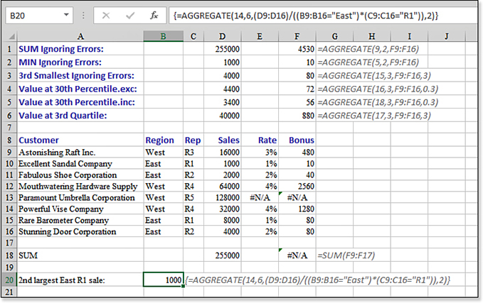
2 or 3 as the options argument for AGGREGATE allows the function to ignore error cells in a range.You can also use the function to ignore cells hidden by a filter. Whereas the old SUBTOTAL function enabled you to do this for 11 calculation functions, the AGGREGATE function adds 8 new functions to the list.
Table 8.5 shows the 19 functions available in the AGGREGATE function. This list mirrors the 11 functions available in SUBTOTAL (arranged alphabetically to match those in the SUBTOTAL function) and then 8 new functions arranged in order of popularity.
Table 8.5 Functions Available in AGGREGATE
Fx # |
Function |
|---|---|
1 |
AVERAGE |
2 |
COUNT |
3 |
COUNTA |
4 |
MAX |
5 |
MIN |
6 |
PRODUCT |
7 |
STDDEV.S |
8 |
STDDEV.P |
9 |
SUM |
10 |
VAR.S |
11 |
VAR.P |
12 |
MEDIAN |
13 |
MODE.SNGL |
14 |
LARGE |
15 |
SMALL |
16 |
PERCENTILE.INC |
17 |
QUARTILE.INC |
18 |
PERCENTILE.EXC |
19 |
QUARTILE.EXC |
The last six functions in this list require you to specify a value for k as the fourth argument. LARGE and SMALL typically return the kth largest or smallest value from a list. Use the fourth argument in AGGREGATE to specify the value for k. The last six functions allow for a calculated array instead of a range of cells. After September 2018, customers using Office 365 will be able to specify arrays for all 19 functions within aggregate. Excel 2019 and earlier will allow arrays only for the last six functions.
In cell F3 of Figure 8.2, the final argument of 3 specifies that you want the third smallest number in the array. For LARGE, SMALL, and QUARTILE, you should specify an integer for k. For PERCENTILE, specify a decimal between 0 and 1.
When you are trying to return results from the visible rows of a filtered data set, you can use either SUBTOTAL or AGGREGATE. In Figure 8.3, the SUM function in D1 returns the sum of the visible and hidden rows. The SUBTOTAL function in D2 returns the sum of the visible rows, the same as the AGGREGATE function in D3. The advantage of AGGREGATE is that it can return MEDIAN, LARGE, SMALL, PERCENTILE, and QUARTILE on the visible rows as well.
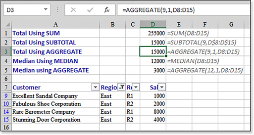
AGGREGATE performs calculations on the visible items of a filtered data set.Choosing Between COUNT and COUNTA
The key to choosing between COUNT and COUNTA is to analyze the data you want to count. In Figure 8.4, someone has used the letter X in column B to indicate that training has been started. In this case, you would use COUNTA to get an accurate count. Column C contains dates (which are treated as numeric). In column C, either COUNT or COUNTA returns the correct result. Column D has a mix of text and numeric entries. If you want to count how many people took the test, use COUNTA. If you want to count how many people received a numeric score, use COUNT.
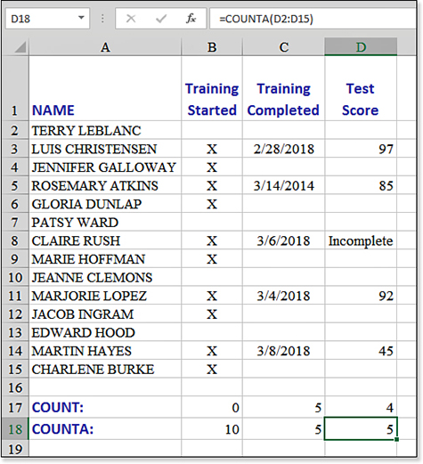
COUNT or COUNTA depends on whether your data is numeric. COUNT counts only dates and numeric entries. COUNTA counts anything that is nonblank.Rounding Numbers
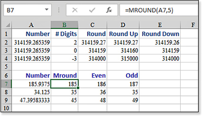
You can use a variety of functions—including ROUND, ROUNDDOWN, ROUNDUP, INT, TRUNC, FLOOR, FLOOR.MATH, CEILING, CEILING.MATH, EVEN, ODD, and MROUND—to round a result or to remove decimals from a result. The most common function is ROUND.
ROUND(number, num_digits)rounds the number. To round to the nearest dollar, use 0 as the second argument. To round to the nearest penny, use 2 as the second argument. To round to the nearest thousand dollars, use –3 as the third argument.ROUNDUP(number, num_digits)always rounds away from zero. Although this usually makes the number larger, the behavior for negative numbers is unusual.=ROUNDUP(-1.1,0)rounds away from zero to –2. If you want that to round to –1, useTRUNC(number)instead.ROUNDDOWN(number, num_digits)always rounds toward zero. Although this makes sense for positive numbers, the result for negative numbers might not make sense.=ROUNDDOWN(-3.1,0)rounds toward zero and produces –3. If you expect this to produce –4, use=INT(-3.1)instead.MROUND(number, multiple)rounds to the nearest multiple. Use for rounding to the nearest 5 or 25.=MROUND(115,25)rounds to 125. There are some unusual variants.=EVEN(number)always rounds up to an even number, for the unusual situation in which items are packed two to a case.=ODD(number)rounds up to an odd integer.
Figure 8.5 illustrates several rounding options.
The last four functions in this group—CEILING, CEILING.MATH, FLOOR, and FLOOR.MATH—round a number in a certain direction to a certain number of digits. They require you to enter the number and the number of decimals to which to round. The behavior of the functions when a number was negative caused complaints from the mathematics community, so the Excel team reversed the behavior with the .MATH versions of the functions.
For example, =CEILING(5.1,1) rounds the 5.1 up to 6. Originally, Excel would always round away from zero: =CEILING(-5.1,-1) would round to –6. Mathematicians pointed out that –6 is actually lower than 5.1 and the correct answer should be –5. Thus, CEILING.MATH(-5.1,1) rounds up to –5.
The older CEILING function required the second argument to have the same sign as the first argument. The .MATH versions can deal with a negative number and a positive significance. Microsoft added an optional third Mode argument that allows CEILING.MATH to round away from zero. Figure 8.6 illustrates CEILING.
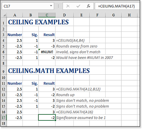
CEILING.MATH rounds toward zero.Using SUBTOTAL Instead of SUM with Multiple Levels of Totals
Consider the data set shown in Figure 8.7. This report shows a list of invoices for each customer. Someone has manually inserted rows and used the SUM function to total each customer. Cells C70 and C75 contain a SUM function.
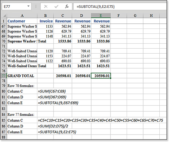
SUBTOTAL instead of SUM for the customer totals, the problem of creating a grand total becomes simple.It becomes incredibly difficult to total the data when it has intermediate SUM functions. The original formula in C77 must point to each subtotal cell.
Many accountants can teach you the old accounting trick whereby you total the entire column and divide by two to get the grand total. This is based on the assumption that every dollar is in the column twice: once on the detail row and once on the summary row. The formula in D77 is far shorter than the formula in C77 and produces the same answer. This trick does work, but it is hard to explain to your manager why it works.
A better solution is to use the SUBTOTAL function. Instead of =SUM(D2:D75), use =SUBTOTAL(9,D2:D75). The function totals all numbers in D2:D75 but ignores other subtotal functions.
While you are summing in this case, the SUBTOTAL function offers 11 arguments, numbered from 1 to 11: AVERAGE, COUNT, COUNTA, MAX, MIN, PRODUCT, STDEV, STDEVP, SUM, VAR, and VARP. It just happens that SUM is the ninth item in this list when these functions are arranged alphabetically in the English language, so 9 became the function number for SUM.
Totaling Visible Cells Using SUBTOTAL
If you are using a filter to query a data set, you can use the SUBTOTAL function instead of the SUM function to show the total of the visible rows. In Figure 8.8, cell E1 contains a SUM function, which totals rows whether they are visible or not. Cell E2 contains a SUBTOTAL function. As you use the Filter drop-down menus to show just rows for sales of J730 by Jamie, the SUBTOTAL function updates to reflect the total of the visible rows. This makes the SUBTOTAL function a great tool for ad-hoc reporting.
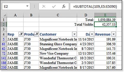
SUBTOTAL function in cell E2 ignores rows hidden as the result of a filter.Note
Although the function in Figure 8.8 uses the function number 109, the Subtotal command always ignores rows hidden as the result of a filter. =SUBTOTAL(9,E5:E5090) would return an identical result when the rows are hidden through a filter, as in this case. If you have rows hidden by the Hide command, you should use 109 to ignore the manually hidden rows.
Using RAND, RANDARRAY, and RANDBETWEEN to Generate Random Numbers and Data
In some situations, you might want to generate random numbers. Excel offers three functions to assist with this process: RAND, RANDARRAY, and RANDBETWEEN.
The RAND function returns an evenly distributed random number greater than or equal to 0 and less than 1. A new random number is returned every time the worksheet is calculated.
=RAND() generates a random decimal between 0 and 0.999999999999999. Whether you are a teacher trying to randomly assign the order for book report presentations or the commissioner of a fantasy football league trying to figure out the draft sequence, =RAND() can help.
Starting in late 2018, Office 365 customers can use the new RANDARRAY([Rows],[Columns] to generate an array of results similar to RAND(). To generate a random number greater than or equal to 0 but less than 100, you can use RAND()*100.
To generate a random sequence for a list, you select a blank column next to your data and enter =RAND() in the column. Every time you press the F9 key, the column generates a new set of random numbers. You might want to agree up front with the draft participants that you will press F9 three times to randomize the list and then convert the formulas to values. To do so, follow these steps:
Enter the heading
Randomin row 1 next to your data.Enter
=RAND()in cell B2.Move the cell pointer to cell B2 and double-click the fill handle.
Turn off automatic calculation by using Formulas, Calculation Options, Manual. This prevents the
RAND()functions from recalculating after you sort in step 7.Press the F9 key three times.
Choose one cell in column B.
From the Data tab, click the AZ button to sort ascending. The new sequence of items in column A is random (see Figure 8.9).
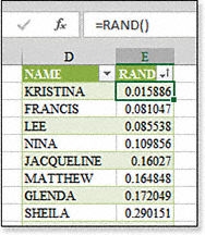
Figure 8.9 Kristina gets to draft first in this season’s fantasy football league, thanks to the RANDfunction.
You can also use this technique to select a random subset from a data set. If your manager wants you to contact every 20th customer, you can select all the customers in which =RAND() is 0.05 or less.
Whereas =RAND() returns a random decimal, =RANDBETWEEN generates an integer between two integers.
The RANDBETWEEN function returns a random integer between the numbers you specify. A new random number is returned every time the worksheet is calculated. This function takes the following arguments:
bottom—This is the smallest integerRANDBETWEENcan return.top—This is the largest integerRANDBETWEENcan return.
To generate random numbers between 50 and 59, inclusive, you use =RANDBETWEEN(50,59). RANDBETWEEN is easier to use than =RAND to achieve random integers; with =RAND, you would have to use =INT(RAND()*10)+50 to generate this same range of data.
Even though RANDBETWEEN generates integers, you can use it to generate sales prices or even letters. =RANDBETWEEN(5000,9900)/100 generates random prices between $50.00 and $99.00, including prices with cents, such as $76.54.
The capital letter A is also known as character 65 in the ASCII character set. B is 66, C is 67, and so on up through Z, which is character 90. You can use =CHAR(RANDBETWEEN(65,90)) to generate random capital letters.
Choosing a Random Item from a List
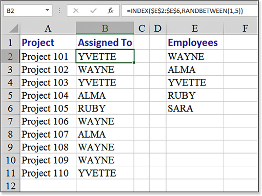
In Figure 8.10, you want to randomly assign employees to certain projects. The list of projects is in column A. The list of employees is in E2:E6. As shown in Figure 8.10, the function for B2:B11 is =INDEX($E$2:$E$6,RANDBETWEEN(1,5)).
Using =ROMAN to Finish Movie Credits and =ARABIC to Convert Back to Digits
Excel can convert numbers to Roman numerals. If you stay in the theater after a movie until the end of movie credits, you see that the copyright date is always expressed in Roman numerals. If you are the next J.J. Abrams, you can use =ROMAN(2022) or =ROMAN(YEAR(Now())) to generate such a numeral.
Note
Romans did have a way to represent 5,000 and 10,000, but the format cannot be typed on a modern keyboard; hence, the programmers behind ARABIC are apparently allowing nonsensical numbers like MMMMMIV.
The =ARABIC() function can convert a Roman numeral back to a regular number. Whereas =ROMAN() works only with the numbers 1 through 3,999, the ARABIC function deals with invalid Roman numerals from –255,000 through 255,000. Leviculus!
Using ABS to Figure Out the Magnitude of Error
Suppose that you work for a local TV station, and you want to prove that your forecaster is more accurate than those at the other stations in town. The forecaster at the rival station in town is horrible—some days he misses high, and other days he misses low. The rival station uses Figure 8.11 to say that his average forecast is 99 percent accurate. All those negative and positive errors cancel each other out in the average.
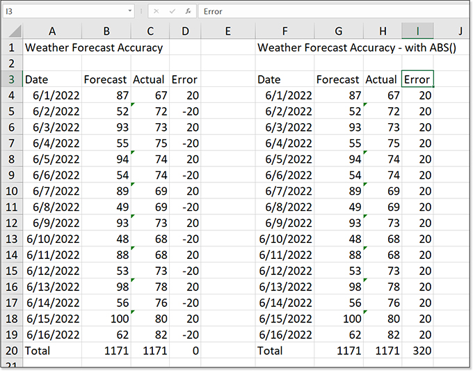
The ABS function measures the size of the error. Positive errors are reported as positive, and negative errors are reported as positive as well. You can use =ABS(A2-B2) to demonstrate that the other station’s forecaster is off by 20 degrees on average.
Using GCD and LCM to Perform Seventh-Grade Math
My seventh-grade math teacher, Mr. Irwin, taught me about greatest common denominators and least common multiples. For example, the least common multiple of 24 and 36 is 72. The greatest common denominator of 24 and 36 is 12. I have to admit that I never saw these concepts again until my son Josh was in seventh grade. This must be permanently part of the seventh-grade curriculum.
If you are in seventh grade or you are assisting a seventh grader with his or her math lesson, you will be happy to know that Excel can calculate these values for you.
Syntax:
=GCD(number1,number2,...)
The GCD function returns the greatest common divisor of two or more integers. The greatest common divisor is the largest integer that divides both number1 and number2, and so on, without a remainder.
The arguments number1, number2,... are 1 to 255 values. If any value is not an integer, it is truncated. If any argument is nonnumeric, GCD returns a #VALUE! error. If any argument is less than zero, GCD returns a #NUM! error. The number 1 divides any value evenly. A prime number has only itself and 1 as even divisors.
Syntax:
=LCM(number1,number2,...)
The LCM function returns the least common multiple of integers. The least common multiple is the smallest positive integer that is a multiple of all integer arguments—number1, number2, and so on. You use LCM to add fractions with different denominators.
The arguments number1, number2,... are one to 255 values for which you want the least common multiple. If the value is not an integer, it is truncated. If any argument is nonnumeric, LCM returns a #VALUE! error. If any argument is less than 1, LCM returns a #NUM! error.
Using MOD to Find the Remainder Portion of a Division Problem
The MOD function is one of the obscure math functions that I find myself using quite frequently. Have you ever been in a group activity in which everyone in the group was to count off by sixes? This is a great way to break up a group into six subgroups. It makes sure that friends who were sitting together get put into disparate groups.
Using the MOD function is a great way to perform this concept with records in a database. Perhaps for auditing, you need to check every eighth invoice. Or you need to break up a list of employees into four groups. You can solve these types of problems by using the MOD function.
Think back to when you were first learning division. If you had to divide 43 by 4, you would have written that the answer was 10 with a remainder of 3. If you divide 40 by 4, the answer is 10 with a remainder of 0.
The MOD function divides one number by another and reports back just the remainder portion of the result. You end up with an even distribution of remainders. If you convert the formulas into values and sort, your data is broken into similar-sized groups.
The MOD function returns the remainder after number is divided by divisor. The result has the same sign as divisor. This function takes the following arguments:
number—This is the number for which you want to find the remainder.divisor—This is the number by which you want to dividenumber. Ifdivisoris 0,MODreturns a#DIV/0!error.Note
MODis short for modulo, the mathematical term for this operation. You would normally say that 17 modulo 3 is 2.
The MOD function is good for classifying records that follow a certain order. For example, the SmartArt gallery contains 84 icons arranged with 4 icons per row. To find the column for the 38th icon, use =MOD(38,4).
The example in Figure 8.12 assigns all employees to one of four groups.
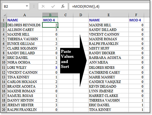
=MOD(ROW(),4). Then paste the values and sort by the remainders.Using SQRT and POWER to Calculate Square Roots and Exponents
Most calculators offer a square root button, so it seems natural that Excel would offer a SQRT function to do the same thing. To square a number, you multiply the number by itself, ending up with a square. For example, 5×5 = 25.
A square root is a number that, when multiplied by itself, leads to a square. For example, the square root of 25 is 5, and the square root of 49 is 7. Some square roots are more difficult to calculate. The square root of 8 is a number between 2 and 3—somewhere close to 2.828. You can calculate the number with =SQRT(8).
A related function is the POWER function. If you want to write the shorthand for 6×6×6×6×6, you would say “six to the fifth power,” or 6^5. Excel can calculate this with =POWER(6,5).
Note
SQRTPI is a specialized version of SQRT. This function is handy for converting square shapes to equivalent-sized round shapes.
Figuring Out Other Roots and Powers
The SQRT function is provided because some math people expect it to be there. There are no equivalent functions to figure out other roots.
If you multiply 5×5×5 to get 125, then the third root of 125 is 5. The fourth root of 625 is 5. Even a $30 calculator offers a key to generate various roots beyond a square root. Excel does not offer a cube root function. In reality, even the POWER and the SQRT functions are not necessary.
=6^3is 6 raised to the third power, which is 6×6×6, or 216.=2^8is 2 to the eighth power, which is 2×2×2×2×2×2×2×2, or 256.
For roots, you can raise a number to a fractional power:
=256^(1/8)is the eighth root of 256. This is 2.=125^(1/3)is the third root of 125. This is 5.
Thus, instead of using =SQRT(25), you could just as easily use =25^(1/2). However, people reading your worksheets are more likely to understand =SQRT(25) than =25^(1/2).
Using SUMIFS, AVERAGEIFS, COUNTIFS, MAXIFS, and MINIFS to Conditionally Calculate
The COUNTIF and SUMIF functions debuted in Excel 97. They would let you sum or count records that met a single condition. Microsoft dramatically improved those functions with updated functions SUMIFS and AVERAGEIFS. The plural version of the functions can handle up to 127 conditions.
In February 2017, Microsoft added MAXIFS and MINIFS to find the smallest or largest value for records that meet one or more conditions.
Figure 8.13 shows a database. You want to examine all of the Central region sales where the product is Widget. If column B says Widget and column C says Central, you want to perform calculations on the revenue in column D. In this figure, the text values Widget and Central are stored in F1 and G1 respectively.
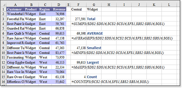
SUMIFS, AVERAGEIFS, MINIFS, MAXIFS, and COUNTIFS calculate only the records that fall in the Central region for product Widget.The SUMIFS function starts with a reference to the revenue amounts in D2:D16. After that first argument, you will provide anywhere from 1 to 127 pairs of arguments. In each pair, the first argument is the range to examine. The second argument is the value to match. For example, to find records in the Central region, you could specify C2:C16,F1. To find records where the product is Widget, you would use B2:B16,G1.
Thus, for a formula to test two conditions, you will have five arguments. The SUMIFS, AVERAGEIFS, MINIFS, and MAXIFS all follow the same syntax. The difference is the COUNTIFS function, which omits the initial argument to specify the numeric column.
Syntax:
SUMIFS(sum_range,criteria_range1,criteria1[,criteria_range2, criteria2...])
The SUMIFS() function adds the cells in a range that meet multiple criteria.
Note the following in this syntax:
sum_rangeis the range to sum.criteria_range1, criteria_range2,...are one or more ranges in which to evaluate the associated criteria.criteria1, criteria2,...are one or more criteria in the form of a number, an expression, a cell reference, or text that define which cells will be added. For example, they can be expressed as32,"32",">32","apples", orB4.Each cell in
sum_rangeis summed only if all the corresponding criteria specified are true for that cell.You can use the wildcard characters question mark (?) and asterisk (*) in
criteria. A question mark matches any single character; an asterisk matches any sequence of characters. If you want to find an actual question mark or asterisk, you need to type a tilde (~) before the character.Unlike the range and criteria arguments in
SUMIF, the size and shape of eachcriteria_rangeandsum_rangemust be the same.
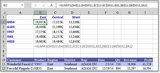
In Figure 8.14, you want to build a table that shows the total by region and product. sum_range is the revenue in H11:H5011. The first criteria pair consists of the regions in $C$11:$C$5011 being compared to the word East in B$1. The second criteria pair consists of the divisions in $B$11:$B$5011 being compared to G854 in $A2. The formula in B2 is =SUMIFS($H$11:$H$5011,$C$11:$C$5011,B$1,$B$11:$B$5011,$A2). You can copy this formula to B2:D6.
SUMIFS() function is used to create this summary by region and product.Dates and Times in Excel
Date calculations can drive people crazy in Excel. If you gain a certain confidence with dates in Excel, you will be able to quickly resolve formatting issues that come up.
Here is why dates are a problem. First, Excel stores dates as the number of days since January 1, 1900. For example, June 30, 2021, is 44,377 days since 1/1/1900. When you enter 6/30/2021 in a cell, Excel secretly converts this entry to 44,377 and formats the cell to display a date instead of the value. So far, so good. The problem arises when you try to calculate something based on the date.
When you try to perform a calculation on two cells when the first cell is formatted as currency and the second cell is formatted as fixed numeric with three decimals, Excel has to decide if the new cell inherits the currency format or the fixed with three decimals format. These rules are hard to figure out. In any given instance, you might get the currency format or the fixed with three decimals format, or you might get the format previously assigned to the cell with the new formula. With numbers, a result of $80.52 or 80.521 looks about the same. You can probably understand either format.
However, imagine that one of the cells is formatted as a date. Another cell contains the number 30. If you add the 30 to the date, which format does Excel use? If the cell containing the new formula happened to be previously assigned a numeric format, the answer suddenly switches from a date format to the numeric equivalent. This is frustrating and confusing. You start with June 30, 2021, add 30 days, and get an answer of 44,407. This makes no sense to an Excel novice. It forces many people to give up on dates and start storing dates as text that looks like dates. This is unfortunate because you can’t easily do calculations on text cells that look like dates.
Here is a general guideline to remember: If you work with dates in the range of the years 2017 to 2028, those numeric equivalents are from 42,736 through 47,118. If you do some date math and get a strange answer in the 40,000–50,000 range, Excel probably has the right answer, but the numeric format of the answer cell is wrong. You need to select Short Date from the Number drop-down menu on the Home tab to correct the format.
The Excel method for storing dates is simple when you understand it. If you have a date cell and need to add 15 days to it, you add the number 15 to the cell. Every day is equivalent to the number 1, and every week is equivalent to the number 7. This is very simple to understand.
When you see 44,377 instead of June 30, 2021, Excel calls the 44,377 a serial number. Some of the Excel functions discussed here convert from a serial number to text that looks like a date, or vice versa.
For time, Excel adds a decimal to the serial number. There are 24 hours in a day. The serial number for 6:00 a.m. is 0.25. The serial number for noon is 0.5. The serial number for 6:00 p.m. is 0.75. The serial number for 3:00 p.m. on June 30, 2021 is 44,377.625. To see how this works, try this out:
Create a blank Excel workbook.
In any cell, enter a number in the range of 40,000 to 45,000.
Add a decimal point and any random digits after the decimal.
Select that cell.
From the Home tab, select the dialog box launcher in the lower-right corner of the Number group.
In the Date category, scroll down and select the format 3/14/01 1:30 PM. Excel displays your random number as a date and time. If the decimal portion of your number is greater than 0.5, the result is in the p.m. portion of the day.
Go to another cell and enter the date you were born, using a four-digit year.
Again, select the cell and format it as a number. Excel converts it to show how many days after the start of the last century you were born. This is great trivia but not necessarily useful.
Caution
Although most Excel date issues can be resolved with formatting, you should be aware of some real date problems:
On a Macintosh, Excel dates are stored since January 1, 1904. If you are using a Mac, your serial number for a date in 2021 will be different from that on a Windows PC. Excel handles this conversion when files are moved from one platform to another.
Excel cannot handle dates in the 1800s or before. This really hacks off all my friends who do genealogy. If your Great-Great-Great Uncle Felix was born on February 17, 1895, you are going to have to store that as text.
Around Y2K, someone decided that 1930 is the dividing line for two-digit years. If you enter a date with a two-digit year, the result is in the range of 1930 through 2029. If you enter 12/31/29, this will be interpreted as 2029. If you enter 1/1/30, it will be interpreted as 1930. If you need to enter a mortgage ending date of 2040, for example, be sure to use the four-digit year, 6/15/2040. If you are regularly entering dates in the 2030–2040 range, you can change the dividing line for two-digit years. Go to Region And Language settings in the Control Panel. Click Additional Settings. Click the Date tab. The When A Two Digit Year Is Entered setting allows you to change the dividing line.
The point is that Excel dates are nothing to be afraid of. You need to understand that behind the scenes, Excel is storing your dates as serial numbers and your times as decimal serial numbers. Occasionally, circumstances cause a date to be displayed as a serial number. Although this freaks some people out, it is easy to fix using the Format Cells dialog box. Other times, when you want the serial number (for example, to calculate elapsed days between two dates), Excel converts the serial number to a date, indicating, for example, that an invoice is past due by “February 15, 1900” days. When you get these types of nonsequiturs, you can visit the Format Cells dialog box. Or press the shortcut key—Ctrl+Shift+tilde—to format the cell as General.
Troubleshooting
For compatibility with ancient spreadsheet programs, Excel includes the date of February 29, 1900—a date that does not exist.
Leap day is not added to the years 1700, 1800, 1900, 2100, 2200, 2300, and 2500. Lotus 1-2-3 erroneously included February 29, 1900. To allow Lotus files to convert to Excel, Microsoft repeated the error. The result is that any weekdays from January 1, 1900, to February 28, 1900, are off by one day.
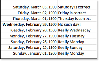
A table of dates formatted as a long date spans from March 3, 1900, back to February 25, 1900. Excel shows that March 1, 1900, is a Thursday, and this is correct. However, Microsoft says the Wednesday before this day is February 29, 1900—a day that does not exist. This causes all weekdays from January 1, 1900, to February 28, 1900, to be wrong in Excel. When Excel says that February 28, 1900, was on a Tuesday, that is incorrect; February 28, 1900, really was a Wednesday.
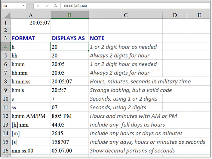
Understanding Excel Date and Time Formats
It is worthwhile to learn the various Excel custom codes for date and time formats. Figure 8.15 shows a table of how March 5, 2021, would be displayed in various numeric formats. The codes in A4:A17 are the possible codes for displaying just date, month, or year. Most people know the classic mm/dd/yyyy format, but far more formats are available. You can cause Excel to spell out the month and weekday by using codes such as dddd, mmmm d, yyyy. Here are the possibilities:
mm—Displays the month with two digits. Months before October are displayed with a leading zero (for example, January is 01).m—Displays the month with one or two digits, as necessary.mmm—Displays a three-letter abbreviation for the month (for example, Jan, Feb).mmmm—Spells out the month (for example, January, February).mmmmm—First letter of the month, useful for creating “JFMAMJJASOND” chart labels.dd—Displays the day of the month with two digits. Dates earlier than the 10th of the month are displayed with a leading zero (for example, the 1st is 01).d—Displays the day of the month with one or two digits, as needed.ddd—Displays a three-letter abbreviation for the name of the weekday (for example, Mon, Tue).dddd—Spells out the name of the weekday (for example, Monday, Tuesday).yyory—Uses two digits for the year (for example, 15).yyyyoryyy—Uses four digits for the year (for example, 2015).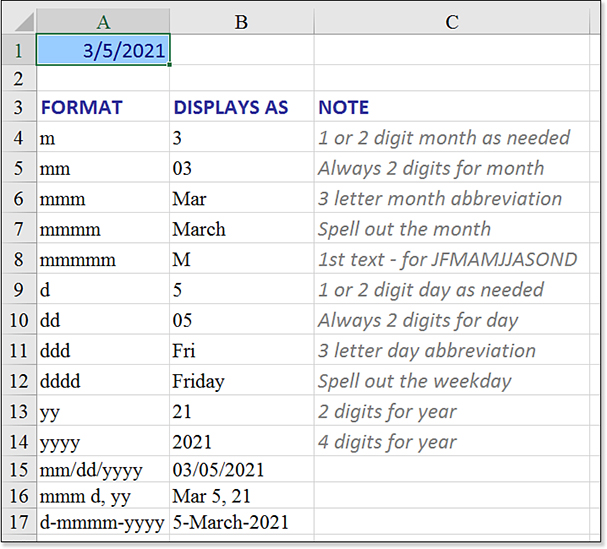
Figure 8.15 Any of these custom date format codes can be typed in the Custom Numeric Format box.
You are allowed to string together any combination of these codes with a space, comma, slash, or dash. It is valid to repeat a portion of the date format. For example, the format dddd, mmmm d, yyyy shows the day portion twice in the date and would display as Thursday, March 5, 2018.
Although the date formats are mostly intuitive, several difficulties exist in the time formats. The first problem is the M code. Excel has already used M to mean month. In a time format, you cannot use M alone to mean minutes. The M code must either be preceded or followed by a colon.
There is another difficulty: When you are dealing with years, months, and days, it is often perfectly valid to mention only one of the portions of the date without the other two. It is common to hear any of these statements:
“I was born in 1965.”
“I am going on vacation in July.”
“I will be back on the 27th.”
If you have a date such as March 5, 2018, and use the proper formatting code, Excel happily tells you that this date is March or 2018 or the 5th. Technically, Excel is leaving out some really important information—the 5th of what? As humans, we can often figure out that this probably means the 5th of the next month. Thus, we aren’t shocked that Excel is leaving off the fact that it is March 2018.
Tip
Custom number formats are entered in the Format Cells dialog box. There are three ways to display this dialog:
Press Ctrl+1.
From the Home tab, in the Number group, select the drop-down menu and select More Number Formats from the bottom of the drop-down menu.
Click the expand icon in the lower-right corner of the Number group on the Home tab.
When the Format Cells dialog box is displayed, you select the Number tab. In the Category list, you select Custom. In the Type box, you enter your custom format. The Sample box displays the active cell with the format applied.
Imagine how strange it would be if Excel did this with regular numbers. Suppose you have the number 352. Would Excel ever offer a numeric format that would display just the tens portion of the number? If you put 352 in a cell, would Excel display 5 or 50? It would make no sense.
Excel treats time as an extension of dates and is happy to show you only a portion of the time. This can cause great confusion. To Excel, 40 hours really means 1 day and 16 hours. If you create a timesheet in Excel and format the total hours for the week as H:MM, Excel thinks that you are purposefully leaving off the day portion of the format! Excel presents 45 hours as just 21 hours because it assumes you can figure out there is 1 day from the context. But our brains don’t work that way; 21 hours means 21 hours, not 1 day and 21 hours.
To overcome this problem in Excel, you use square brackets. Surrounding any time element with square brackets tells Excel to include all greater time/date elements in that one element, as in the following examples:
5 days and 10 hours in
[H]format would be 130.5 days and 10 hours in
[M]format would be 7800, to represent that many minutes.5 days and 10 hours in
[S]format would be 468000, to represent that many seconds.
As shown in Figure 8.16, the time formatting codes include various combinations of h, hh, s, ss, :mm, and mm:, all of which can be modified with square brackets.
To display date and time, you enter the custom date format code, a space, and then the time format code.
Examples of Date and Time Functions
In all the examples in the following sections, you should use care to ensure that the resulting cell is formatted using the proper format, as discussed in the preceding section.
Using NOW and TODAY to Calculate the Current Date and Time or Current Date
There are a couple of keyboard shortcuts for entering date and time. Pressing Ctrl+; enters the current date in a cell. Pressing Ctrl+: enters the current time in a cell. However, both of these hotkeys create a static value; that is, the date or time reflects the instant that you typed the hotkey, and it never changes in the future.
Excel offers two functions for calculating the current date: NOW and TODAY. These functions are excellent for figuring out the number of days until a deadline or how late an open receivable might be.
Caution
It would be nice if NOW() would function like a real-time clock, constantly updating in Excel. However, the result is calculated when the file is opened, with each press of the F9 key, and when an entry is made elsewhere in the worksheet.
Syntax:
=NOW()
=TODAY()
NOW returns the serial number of the current date and time. TODAY returns the serial number of the current date. The TODAY function returns today’s date, without a time attached. The NOW function returns the current date and time.
Both of these functions can be made to display the current date, but there is an important distinction when you are performing calculations with the functions. In Figure 8.17, column A contains NOW functions, and column C contains TODAY functions. Row 2 is formatted as a date and time. Row 3 is formatted as a date. Row 4 is formatted as numeric. Cell A3 and C3 look the same. If you need to display the date without using it in a calculation, NOW or TODAY work fine.
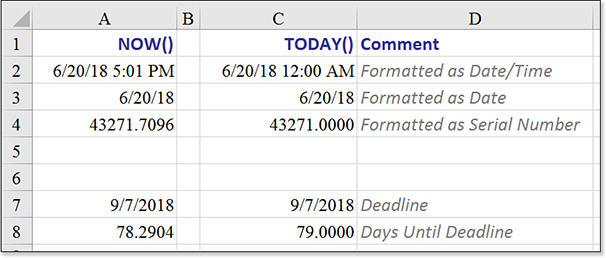
NOW and TODAY can be made to look alike, but you need to choose the proper one if you are going to be using the result in a later calculation.Row 8 calculates the number of days until a deadline approaches. Although most people would say that tomorrow is one day away, the formula in A8 would tend to say that the deadline is 0.2904 days away. This can be deceiving. If you are going to use the result of NOW or TODAY in a date calculation, you should use TODAY to prevent Excel from reporting fractional days. The formula in A8 is =A7-A3, formatted as numeric instead of a date.
Using YEAR, MONTH, DAY, HOUR, MINUTE, and SECOND to Break a Date/Time Apart
If you have a column of dates from the month of July 2018, you can easily make them all look the same by using the MMM-YY format. However, the dates in the actual cells are still different. The July 2018 records are not sorted as if they were a tie. Excel offers six functions that you can use to extract a single portion of the date: YEAR, MONTH, DAY, HOUR, MINUTE, and SECOND.
In Figure 8.18, cell A1 contains a date and time. Functions in A3 through A8 break out the date into components:
=YEAR(date)returns the year portion as a four-digit year.=MONTH(date)returns the month number, from 1 through 12.=DAY(date)returns the day of the month, from 1 through 31.=HOUR(date)returns the hour, from 0 to 23.=MINUTE(date)returns the minute, from 0 to 59.=SECOND(date)returns the second, from 0 to 59.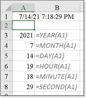
Figure 8.18 These six functions allow you to isolate any portion of a date or time.
In each case, date must contain a valid Excel serial number for a date. The cell containing the date serial number may be formatted as a date or as a number.
Using DATE to Calculate a Date from Year, Month, and Day
The DATE function is one of the most amazing functions in Excel. Microsoft’s implementation of this function is excellent, allowing you to do amazing date calculations.
Syntax:
=DATE(year,month,day)
The DATE function returns the serial number that represents a particular date. This function takes the following arguments:
year—This argument can be one to four digits. Ifyearis between 0 and 1899 (inclusive), Excel adds that value to 1900 to calculate the year. For example,=DATE(100,1,2)returns January 2, 2000 (1900+100). Ifyearis between 1900 and 9999 (inclusive), Excel uses that value as the year. For example,=DATE(2000,1,2)returns January 2, 2000. Ifyearis less than 0 or is 10,000 or greater, Excel returns a#NUM!error.month—This is a number representing the month of the year. Ifmonthis greater than 12,monthadds that number of months to the first month in the year specified. For example,=DATE(1998,14,2)returns the serial number representing February 2, 1999. If zero, it represents December of the previous year. If negative, returns prior months, although –1 represents November, –2 is October, and so on.day—This is a number representing the day of the month. Ifdayis greater than the number of days in the month specified, it adds that number of days to the first day in the month. For example,=DATE(2018,1,35)returns the serial number representing February 4, 2018. Zero represents the last day of the previous month. Negative numbers return days earlier, just as with month. In a trivial example,=DATE(2018,3,5)returns March 5, 2018.
The true power in the DATE function occurs when one or more of the year, month, or day are calculated values. Here are some examples:
If cell A2 contains an invoice date and you want to calculate the day one month later, you use
=DATE(Year(A2),Month(A2)+1,Day(A2)).To calculate the beginning of the month, you use
=DATE(Year(A2),Month(A2),1).To calculate the end of the month, you use
=DATE(Year(A2),Month(A2)+1,1)–1.
The DATE function is amazing because it enables Excel to deal perfectly with invalid dates. If your calculations for Month cause it to exceed 12, this is no problem. For example, if you ask Excel to calculate =DATE(2018,16,45), Excel considers the 16th month of 2018 to be April 2019. To find the 45th day of April 2018, Excel moves ahead to May 15, 2018.
Figure 8.19 shows various results of the DATE and TIME functions.
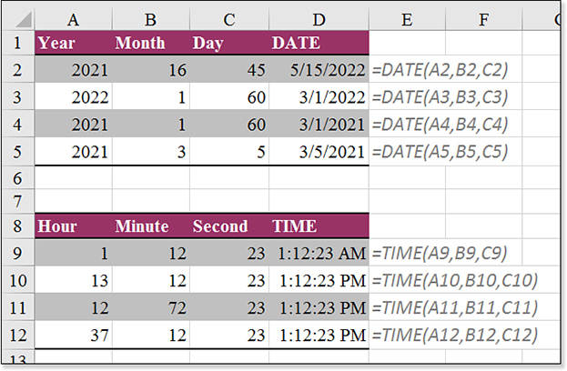
D use DATE or TIME functions to calculate an Excel serial number from three arguments.Using TIME to Calculate a Time
The TIME function is similar to the DATE function. It calculates a time serial number given a specific hour, minute, and second.
Syntax:
=TIME(hour,minute,second)
The TIME function returns the decimal number for a particular time. The decimal number returned by TIME is a value ranging from 0 to 0. 999988425925926, representing the times from 0:00:00 (12:00:00 a.m.) to 23:59:59 (11:59:59 p.m.). This function takes the following arguments:
hour—This is a number from 0 to 23, representing the hour.minute—This is a number from 0 to 59, representing the minute.second—This is a number from 0 to 59, representing the second.
As with the DATE function, Excel can handle situations in which the minute or second argument calculates to more than 60. For example, =TIME(12,72,120) evaluates to 1:14 p.m.
Additional examples of TIME are shown in the bottom half of Figure 8.19.
Using DATEVALUE to Convert Text Dates to Real Dates
It is easy to end up with a worksheet full of text dates. Sometimes this is due to importing data from another system. Sometimes it is caused by someone not understanding how dates work.
If your dates are in many conceivable formats, you can use the DATEVALUE function to convert the text dates to serial numbers, which can then be formatted as dates.
Syntax:
=DATEVALUE(date_text)
The DATEVALUE function returns the serial number of the date represented by date_text. You use DATEVALUE to convert a date represented by text to a serial number. The argument date_text is text that represents a date in an Excel date format. For example, "3/5/2018" and "05-Mar-2018" are text strings within quotation marks that represent dates. Using the default date system in Excel for Windows, date_text must represent a date from January 1, 1900, to December 31, 9999. DATEVALUE returns a #VALUE! error if date_text is out of this range. If the year portion of date_text is omitted, DATEVALUE uses the current year from your computer’s built-in clock. Time information in date_text is ignored.
Any of the text values in column A of Figure 8.20 are successfully translated to a date serial number. In this instance, Excel should have been smart enough to automatically format the resulting cells as dates. By default, the cells are formatted as numeric. This leads many people to believe that DATEVALUE doesn’t work. You have to apply a date format to achieve the desired result.
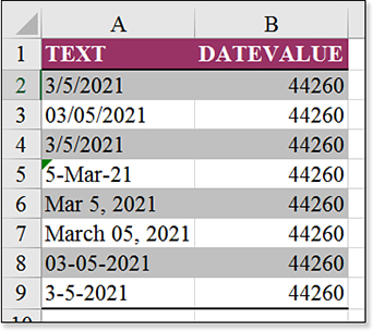
DATEVALUE to convert the text entries in column A to date serial numbers.Caution
The DATEVALUE function must be used with text dates. If you have a column of values in which some values are text, and some are actual dates, using DATEVALUE on the actual dates causes a #VALUE error. You could use =IF(ISNUMBER(A1),A1,DATEVALUE(A1)). Also consider the =DAYS(end,start) function, which deals with either text dates or real dates.
Caution
There are a few examples of text that DATEVALUE cannot recognize. One common example is when there is no space after the comma. For example, “January 21,2011” returns an error. To solve this particular problem, use Replace to change a comma to a comma space.
Using TIMEVALUE to Convert Text Times to Real Times
It is easy to end up with a column of text values that look like times. Similar to using DATEVALUE, you can use the TIMEVALUE function to convert these to real times.
Syntax:
=TIMEVALUE(time_text)
The TIMEVALUE function returns the decimal number of the time represented by a text string. The decimal number is a value ranging from 0 to 0. 999988425925926, representing the times from 0:00:00 (12:00:00 a.m.) to 23:59:59 (11:59:59 p.m.). The argument time_text is a text string that represents a time in any one of the Microsoft Excel time formats. For example, "6:45 PM" and "18:45" are text strings within quotation marks that represent time. Date information in time_text is ignored.
The TIMEVALUE function is difficult to use because it is easy for a person to enter the wrong formats. In Figure 8.21, many people would interpret cell A8 as meaning 45 minutes and 30 seconds. Excel, however, treats this as 45 hours and 30 minutes. This misinterpretation makes TIMEVALUE almost useless for a column of cells that contain a text representation of minute and seconds.
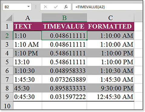
TIMEVALUE to convert the text entries in column A to times. If there is no leading zero before entries with minutes and seconds, the formula produces an unexpected result.Caution
There are a few examples of text that TIMEVALUE cannot recognize. One common example is when there is no space before the AM or PM. For example, “11:00PM” returns an error. To solve this particular problem, use Replace to change “PM” to “ PM” and to change “AM” to “ AM.”
Frustratingly, Excel does not automatically format the results of this function as a time. Column B shows the result as Excel presents it. Column C shows the same result after a time format has been applied.
Using WEEKDAY to Group Dates by Day of the Week
The WEEKDAY function would not be so intimidating if people could just agree how to number the days. This one function can give eight different results, just for Monday.
Syntax:
=WEEKDAY(serial_number,return_type)
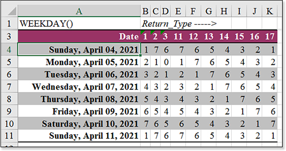
The WEEKDAY function returns the day of the week corresponding to a date. The day is given as an integer, ranging from 1 (Sunday) to 7 (Saturday), by default. This function takes the following arguments:
serial_number—This is a sequential number that represents the date of the day you are trying to find. Dates may be entered as text strings within quotation marks (for example,"1/30/2018","2018/01/30"), as serial numbers (for example, 43130, which represents January 30, 2018), or as results of other formulas or functions (for example,DATEVALUE("1/30/2018")).return_type—This is a number that determines the type of return value:If
return_typeis1or omitted,WEEKDAYworks like the calendar on your wall. Typically, calendars are printed with Sunday on the left and Saturday on the right. The default version ofWEEKDAYnumbers these columns from 1 through 7.If
return_typeis2, you are using the biblical version ofWEEKDAY. In the biblical version, Sunday is the seventh day. Working backward, Monday must occupy the 1 position.If
return_typeis3, you are using the accounting version ofWEEKDAY. In this version, Monday is assigned a value of0, followed by1for Tuesday, and so on. This version makes it very easy to group records by week. If cell A2 contains a date, thenA2-WEEKDAY(A2,3)converts the date to the Monday that starts the week.return_types of11through17were added in Excel 2010.11returns Monday as 1 and Sunday as 7 (the same as using 2).12returns Tuesday as 1,13returns Wednesday as 1, and so on, up to17returning Sunday as 1.
Figure 8.22 shows the results of WEEKDAY for all ten return types.
WEEKDAY function for the ten different return_type values shown in row 3.Using WEEKNUM or ISOWEEKNUM to Group Dates into Weeks
For many versions, Excel did not calculate weeks to match the ANSI standard. The return_type of 21 or the ISOWEEKNUM function returns the week number to match the ANSI standard. In this system, weeks always start on Monday. The first week of the year must have four days that fall into this year. Another way to say this is that the week containing the first Thursday of the month is numbered as Week 1.
In the ANSI system, you might have Week 1 actually starting as early as December 29 or as late as January 4. The last week of the year is numbered 52 in most years but is 53 every fourth year. This system ensures that a year is made up of whole seven-day weeks. This is better than the old results of WEEKNUM.
In the old system with WEEKNUM, the week containing the first of the year was always labeled as Week 1. If the first fell on a Sunday, and your weeks started on Monday, then Sunday, January 1 is Week 1 and Monday, January 2 is Week 2. The possibility of having weeks that last for one day made it difficult to compare one week to the next. Nonetheless, the Excel team added new return_types for this system as well. In the past, 1 meant weeks started on Sunday, and 2 meant weeks started on Monday. Now, you can specify weeks should start on Monday (11), Tuesday (12), and so on, up to Sunday (17).
Syntax:
=WEEKNUM(serial_num,[return_type])
The WEEKNUM function returns a number that indicates where the week falls numerically within a year. This function takes the following arguments:
serial_num—This is a date within the week.return_type—This is a number that determines on what day the week begins. The default is1. Ifreturn_typeis1or omitted, the week begins on Sunday. Ifreturn_typeis2, the week begins on Monday.return_types of11through17were added to Excel 2013 and specify that the week should start on Monday (11) through Sunday (17). The newreturn_typeof21ensures that every week has exactly seven days. Weeks always start on Monday, but the first Thursday of the year is the middle of Week 1.
Calculating Elapsed Time
If you work in a human resources department, you might be concerned with years of service to calculate a certain benefit. Excel provides one function, YEARFRAC, that can calculate decimal years of service in five ways. An old function, DATEDIF (pronounced Date Dif), has been hanging around since Lotus 1-2-3; it can calculate the difference between two dates in complete years, months, or days. Excel 2013 added the DAYS function, which can calculate elapsed days even if one or both of the values are text dates.
Syntax:
=DATEDIF(start_date,end_date,unit)
The DATEDIF function calculates complete years, months, or days. This function calculates the number of days, months, or years between two dates. It is provided for compatibility with Lotus 1-2-3. This function takes the following arguments:
start_date—This is a date that represents the first, or starting, date of the period.end_date—This is a date that represents the last, or ending, date of the period.unit—This is the type of information you want returned. The various values forunitare shown in Table 8.6.Table 8.6 Unit Values Used by the
DATEDIFFunctionUnit Value
Description
Y
The number of complete years in the period. A complete year is earned on the anniversary date of the employee’s start date.
M
The number of complete months in the period. This number is incremented on the anniversary date. If the employee was hired on January 18, that person has earned 1 month of service on the 18th of February. If an employee is hired on January 31, then she earns credit for the month when she shows up for work on the 1st after any month with fewer than 31 days.
D
The number of days in the period. This could be figured out by simply subtracting the two dates.
MD
The number of days, ignoring months and years. You could use a combination of two DATEDIF functions—one using M and one using MD—to calculate days.
YM
The number of months, ignoring years. You could use a combination of two DATEDIF functions—one using Y and one using YM—to calculate months.
YD
The number of days, ignoring complete years.
Figure 8.23 compares the six unit values of DATEDIF. Each cell uses $A$1 as the start date and that row’s column A as the end date.
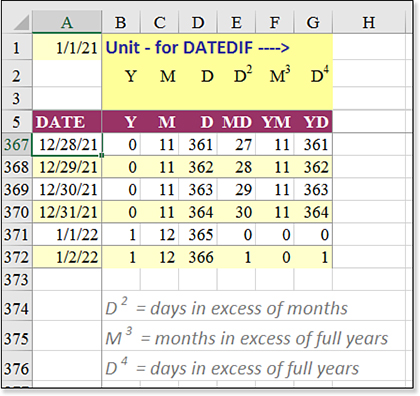
DATEDIF is great for calculating elapsed years, months, and days.Caution
DATEDIF has been in Excel forever, but it was only documented in Excel 2000. Why doesn’t Microsoft reveal DATEDIF in Help? Probably because of the strange anomaly when you try to calculate the gap from the 31st of January to the 1st of March in a non-leap year.
The “
D” version ofDATEDIFreports this as 29 days. This is correct.The “
M” version ofDATEDIFreports this as one full month. This must be correct because the dates span the entire month of February.The “
MD” version ofDATEDIFreports this as a negative two days more than a full month. See cell D7 in Figure 8.24. This is the downside of trying to express a measurement in months when the length of a month is not constant. Negative values for this version ofDATEDIFhappen only when the end date is March 1 or March 2.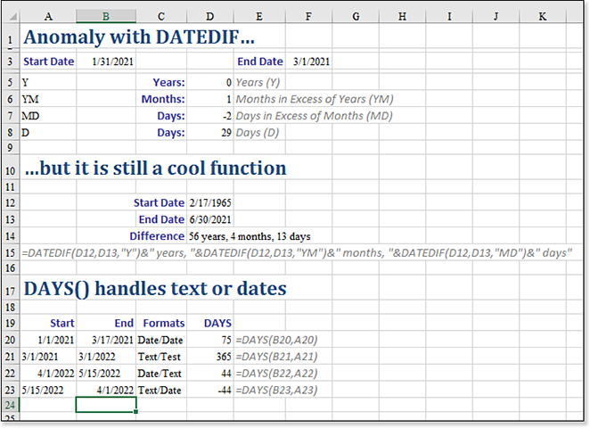
Figure 8.24 In rare cases, DATEDIFwill report 1 month and –2 days.
Despite this problem, for 363 days a year, DATEDIF remains an effective way to express a date delta as a certain number of years, months, and days.
Syntax:
=DAYS(end_date, start_date,)
The DAYS function always calculates elapsed days between two dates. Introduced in Excel 2013, the function offers one new trick: It works with text dates as well as real dates. This function takes the following arguments:
end_date, start_date—The two dates between which you want to know the number of days. If either argument is text, that argument is passed throughDATEVALUE()to return a date.
Using EOMONTH to Calculate the End of the Month
Syntax:
=EOMONTH(start_date,months)
The EOMONTH function returns the serial number for the last day of the month that is the indicated number of months before or after start_date. You use EOMONTH to calculate maturity dates or due dates that fall on the last day of the month. This function takes the following arguments:
start_date—This is a date that represents the starting date.months—This is the number of months before or afterstart_date. A positive value formonthsyields a future date; a negative value yields a past date. Ifmonthsis not an integer, it is truncated.=EOMONTH(A2,0)converts any date to the end of the month.Caution
You must format the result of the
EOMONTHformula to be a date to see the expected results.
Using WORKDAY or NETWORKDAYS or Their International Equivalents to Calculate Workdays
The functions WORKDAY and NETWORKDAYS are pretty cool. They calculate days by excluding weekends and holidays. Weekends can be any two-day period, such as Saturday/Sunday or Thursday/Friday, or any one day, such as only Sunday. As of Excel 2013, you can specify odd work weeks such as Monday, Thursday, Friday, Saturday.
These functions are great for calculating shipping days when you ship with FedEx or UPS. They are also great for making sure your result doesn’t fall on a bank holiday. Here’s how you do it:
In an out-of-the-way section of a spreadsheet, enter any holidays that will fall during the workweek. This might be federal holidays, floating holidays, company holidays, and so on. The list of holidays can either be entered down a column or across a row. In the top portion of Figure 8.25, the holidays are in E2:E11.
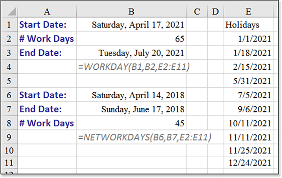
Figure 8.25 WORKDAYandNETWORKDAYScan calculate the number of Monday-through-Friday days, exclusive of a range of holidays.Enter a starting date in a cell, such as B1.
In another cell, enter the number of workdays that the project is expected to take, such as B2.
Enter the ending date formula as
=WORKDAY(B1,B2,E2:E7).
The NETWORKDAYS function takes two dates and figures out the number of workdays between them. For example, you might have a project that is due on June 17, 2018. If today is April 14, 2018, NETWORKDAYS can calculate the number of workdays until the project is due.
Syntax:
=WORKDAY(start_date,days,holidays)
Syntax:
=NETWORKDAYS(start_date,end_date,holidays)
The NETWORKDAYS function returns the number of whole workdays between start_date and end_date. Workdays exclude weekends and any dates identified in holidays. You use NETWORKDAYS to calculate employee benefits that accrue based on the number of days worked during a specific term. This function takes the following arguments:
start_date—This is a date that represents the start date.end_date—This is a date that represents the end date.holidays—This is an optional range of one or more dates to exclude from the working calendar, such as state and federal holidays and floating holidays. The list can be either a range of cells that contain the dates or an array constant of the serial numbers that represent the dates. If any argument is not a valid date,NETWORKDAYSreturns a#NUM!error.
Both of the functions described in this section assume that Saturday and Sunday are weekends and are not workdays. If you have any other weekend system, you can use WORKDAY.INTL or NETWORKDAYS.INTL, as described in the next section.
In Figure 8.25, the current date is entered in cell B6. The project due date is entered in cell B7. The holidays range is in E2:E11, as in the previous example. The formula in cell B8 to calculate workdays is =NETWORKDAYS(B6,B7,E2:E11).
Using International Versions of WORKDAY or NETWORKDAYS
Two functions introduced in Excel 2010 expand the WORKDAY and NETWORKDAYS functions for situations in which the work week is not Monday through Friday. The most common example is a weekend on Friday and Saturday, which has become popular in Qatar, Bahrain, Kuwait, United Arab Emirates, and Algeria. It also handles the situation in which a manufacturing plant is working six days and the weekend is only Sunday. A new form of the weekday argument introduced in Excel 2013 allows for a nonstandard workweek, such as those found at farm markets or barbershops.
Syntax:
=WORKDAY.INTL(start_date,days,weekend,holidays)
Syntax:
=NETWORKDAYS.INTL(start_date,end_date,weekend,holidays)
Both functions work as their noninternational equivalents, with the addition of having the weekend specified as shown below. (Note that there are no noninternational equivalents for 8, 9, and 10.)
1—Weekend on Saturday and Sunday
2—Weekend on Sunday and Monday
3—Weekend on Monday and Tuesday
4—Weekend on Tuesday and Wednesday
5—Weekend on Wednesday and Thursday
6—Weekend on Thursday and Friday
7—Weekend on Friday and Saturday
11—Sunday only
12—Monday only
13—Tuesday only
14—Wednesday only
15—Thursday only
16—Friday only
17—Saturday only
You can specify any nonstandard workweek by using a seven-digit binary text as the weekend argument. The seven digits correspond to Monday through Sunday in order. A 1 indicates the company is closed that day (that is, it is a weekend), and a 0 indicates the company is open.
For example, the Hartville Marketplace is open Monday, Thursday, Friday, and Saturday. The weekend argument would be “0110001”, as shown in Figure 8.26.
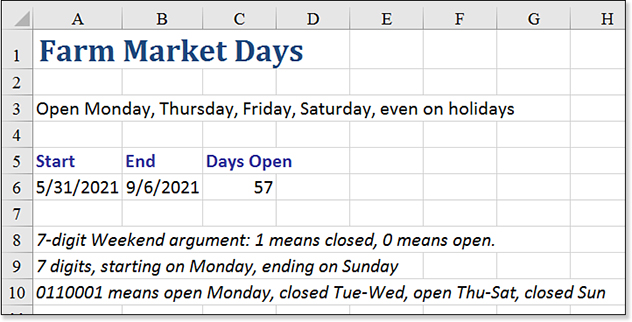
weekday argument to handle nonstandard work weeks.Examples of Text Functions
When they think of Excel, most people think of numbers. Excel is great at dealing with numbers, and it lets you write formulas to produce new numbers. Excel offers a whole cadre of formulas for dealing with text.
You might sometimes be frustrated because you receive data from other people, and the text is not in the format you need. Or the mainframe might send customer names in uppercase, or the employee in the next department might put a whole address into a single cell. Excel provides text functions to deal with all these situations and more.
Joining Text with TEXTJOIN
Microsoft introduced two new functions for joining text in February 2017. The CONCAT function will join text in several cells. While CONCAT is better than the legacy CONCATENATE, it is not as flexible as the amazing TEXTJOIN function.
In Figure 8.27, CONCAT successfully joins a long list of names. However, there is no space or comma between each item. The TEXTJOIN function lets you specify a delimiter. In D6 of the figure, =TEXTJOIN(“, “,True,A2:A24) joins all of the names, and each name is separated by a comm and a space.
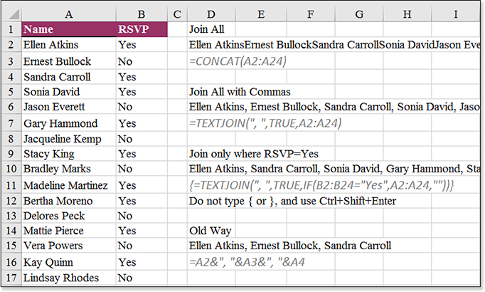
Further, the third argument of TEXTJOIN can be an array or a 3-D reference. That means you can make choices about whether to include each name or not. To join only the names where column B indicates the RSVP is Yes, you could use =TEXTJOIN(“, “,True,IF(B2:B24=”Yes”,A2:A24,””)) entered with Ctrl+Shift+Enter.
Syntax:
=TEXTJOIN(delimiter,ignore_empty,text1,[text2,...])
The TEXTJOIN function joins a list or a range of text using a delimiter.
Before the introduction of TEXTJOIN in 2017, you would have had to use =A2&” “&A3&” “&A4& and so on. Even the legacy CONCATENATE function could not accept a range of cells. The formula would have been =CONCATENATE(“A2”,” “,A3,” “,A4,” “,…).
Using LOWER, UPPER, or PROPER to Convert Text Case
Three functions—LOWER, UPPER, and PROPER—convert text to or from capital letters. In Figure 8.28, the products in column B were entered in a haphazard fashion. Some products used lowercase, and some products used uppercase. Column C uses =UPPER(B2) to make all the products a uniform uppercase.
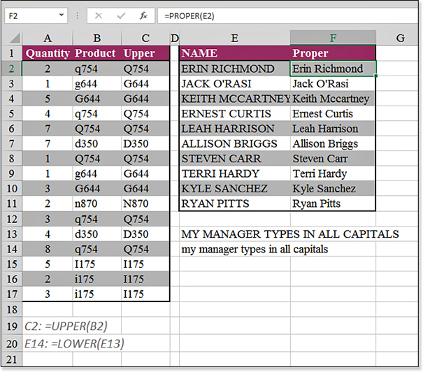
UPPER, LOWER, and PROPER can convert text to and from capital letters.In cell E13, the text was entered by someone who never turns off Caps Lock. You can convert this uppercase to lowercase with =LOWER(E13).
In column E, you see a range of names in uppercase. You can use =PROPER(E2) to convert the name to the proper case, which capitalizes just the first letter of each word. The PROPER function is mostly fantastic, but there are a few cells that you have to manually correct. PROPER correctly capitalizes names with apostrophes, such as O’Rasi in cell F3. It does not, however, correctly capitalize the interior c in McCartney in cell F4. The function is also notorious for creating company names such as Ibm, 3m, and Aep.
Note
If you want to keep the data only in column C, you have to convert the formulas to values before deleting columns A and B. To do this, select the data in column C and then press Ctrl+C to copy. Then select Home, Paste, Paste Values to convert the formulas to values.
Syntax:
=LOWER(text)
The LOWER function converts all uppercase letters in a text string to lowercase. The argument text is the text you want to convert to lowercase. LOWER does not change characters in text that are not letters.
Syntax:
=PROPER(text)
The PROPER function capitalizes the first letter in a text string and any other letters in text that follow any character other than a letter. It converts all other letters to lowercase letters.
The argument text is text enclosed in quotation marks, a formula that returns text, or a reference to a cell containing the text you want to capitalize partially.
Syntax:
=UPPER(text)
The UPPER function converts text to uppercase. The argument text is the text you want to be converted to uppercase. text can be a reference or text string.
Using TRIM to Remove Leading and Trailing Spaces
If you frequently import data, you might be plagued with a couple of annoying situations. This section and the next one deal with those situations.
You may have trailing spaces at the end of text cells. Although " ABC" and "ABC " might look alike when viewed in Excel, they cause functions such as MATCH and VLOOKUP to fail. TRIM removes leading and trailing spaces.
In Figure 8.29, you can see a simple VLOOKUP in column B. The formula in cell B2 is =VLOOKUP(A2,$F$2:$G$5,2,FALSE). Even though you can clearly see that M40498 is in the lookup table, VLOOKUP returns an #N/A! error, which indicates that the product ID is missing from the lookup table.
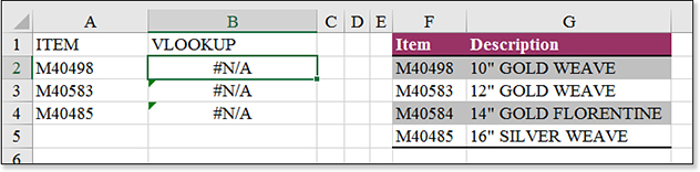
VLOOKUP should work, but in this instance, it fails.To diagnose and correct this problem, follow these steps:
Select one of the data cells in column F. Press the F2 key to put the cell in Edit mode. A flashing insertion character appears at the end of the cell. Check to see if the flashing cursor is immediately after the last character.
Select one of the data cells in column A. Press the F2 key to put the cell in Edit mode. Note whether the flashing insertion character is immediately after the last character. Figure 8.30 shows that the products in column A have several trailing spaces after them. The products in the lookup table do not have any trailing spaces.
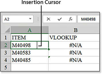
Figure 8.30 Spaces are padding the right side of the products in column A. If the problem is occurring in the values being looked up, you could modify the formula in cell B2 to use the
TRIMfunction. The new formula would be=VLOOKUP(TRIM(A2),$F$2:$G$5,2,FALSE). Figure 8.31 shows how this solves the problem.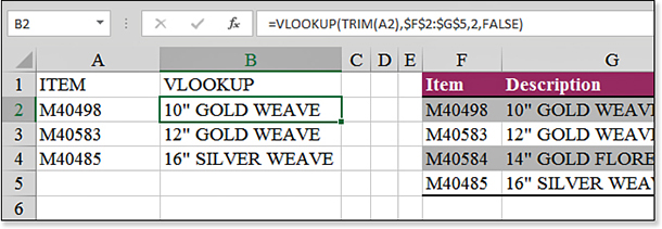
Figure 8.31 Using TRIMto remove leading spaces allowsVLOOKUPto work.If the problem is occurring in the first column of the lookup table, insert a new temporary column. Enter the function
=TRIM(F2)in the temporary column. Copy this formula down to all rows of the lookup table. Copy the new formulas. Select F2. Select Home, Paste, Values to paste the new values. Although the old and new values look the same, theTRIMfunction has removed the trailing spaces, and now the products match.Note
It is not necessarily efficient to calculate, but you can solve the trailing spaces in column F by using
=VLOOKUP(A2,TRIM(F$2:G$5),2,FALSE)if you press Ctrl+Shift+Enter to accept the formula.
Syntax:
=TRIM(text)
The TRIM function removes all spaces from text except for single spaces between words. You use TRIM on text that you have received from another application that might have irregular spacing. The argument text is the text from which you want spaces removed.
In Figure 8.32, cell C1 contains six letters: ABC DEF. You might assume that the cell is set to be centered. However, the formula in cell C2 appends an asterisk to each end of the value in cell C1. This formula shows that there are several leading and trailing spaces in the value.
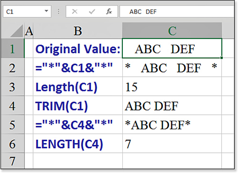
TRIM removes leading spaces and extra interior spaces.Using =LEN(C1) shows that the text actually contains 15 characters instead of six characters. The TRIM(C1) formula removes any leading spaces, any trailing spaces, and any extra interior spaces. The function still leaves one space between ABC and DEF because you want to continue to have words separated by a single space.
The formulas in cells C5 and C6 confirm that the leading and trailing spaces are removed and that the length of the new value is only seven characters.
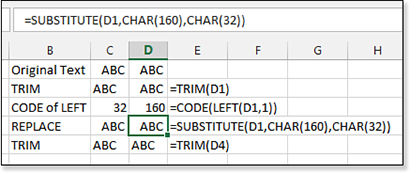
Using the CHAR or UNICHAR Function to Generate Any Character
Early computers used a character set of 128 ASCII characters. Any computer that you’ve had in your home offered at least an 8-bit processor and could easily display 255 characters. Thus, computers sold in the United States offered the original 128 ASCII characters and an extended 128 characters with accented characters needed for German, French, and some other European languages. The CHAR() function makes it possible to display any of these 255 characters.
Today, the Unicode character set includes more than 137,000 characters, covering most written languages used on Earth. Unicode includes glyphs used in languages from Aboriginal to Yijing. You will find glyphs from Braille, Burmese, Cherokee, Greek, Old Persian, and many languages that you have not heard of. There are also map symbols, playing card symbols, emoticons, dice, domino, and mahjong markings. Unfortunately, the Unicode organization officially rejected including Klingon in 2001. Also, although the Calibri font will render chess, dice, and playing card symbols, it does not support domino or mahjong.
All versions of Excel supported CHAR() to generate symbols 0 through 255. Excel 2013 added support for UNICHAR() to render the 100,000+ symbols defined by Unicode.
You might have ventured into Start, All Programs, Accessories, System Tools, Character Map to find a particular character in the Wingdings character set. Also, if you have a favorite symbol, you might have memorized that you can insert the symbol by using a hotkey. For example, if you hold down Alt, type 0169 on the numeric keypad, and then release Alt, an Office program inserts the copyright symbol (©).
Tip
Although I know a few characters off the top of my head, I usually take a look at all characters in a set by entering =CHAR(ROW()) in cells A1:A255. This returns character A in row 65, and so on. In Excel 2019, you can use =UNICHAR(ROW()) in column A1:A1048576 to browse for symbols. To find something in particular, check out https://unicode-table.com/en/#control-character.
Syntax:
=CHAR(number)
The CHAR function returns the character specified by a number. You use CHAR to translate code page numbers you might get from files on other types of computers into characters.
The argument number is a number between 1 and 255 that specifies which character you want. The character is from the character set used by your computer.
Syntax:
=UNICHAR(number)
The UNICHAR function returns the Unicode character specified by a number.
Figure 8.33 shows some symbols available from CHAR and UNICHAR.
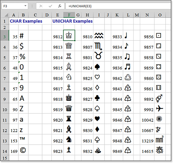
CHAR and UNICHAR results.If you see a strange character in your data, you can learn the character number by using the CODE or UNICODE function, as described in the following section.
Using the CODE or UNICODE Function to Learn the Character Number for Any Character
If you can’t remember that a capital A is character code 65, you can use the CODE function to learn the code associated with the character. The function returns the ASCII code for the first character in the text. =CODE("A") returns 65.
The old CHAR function did not work with characters beyond the first 255 characters. Starting in Excel 2013, the Excel team added the UNICODE function to return the Unicode character number for a character.
Syntax:
=CODE(text)
=UNICODE(text)
The CODE function returns a numeric code for the first character in a text string. The returned code corresponds to the character set used by your computer. The argument text is the text for which you want the code of the first character. This is an important distinction. CODE returns the code for only the first character in a cell. =CODE("A") and =CODE("ABC") return only 65 to indicate the capital letter A.
The UNICODE function returns the character code for the 100,000+ characters currently defined.
Using LEFT, MID, or RIGHT to Split Text
One of the newer rules in information processing is that each field in a database should contain exactly one piece of information. Throughout the history of computers, there have been millions of examples of people trying to cram many pieces of information into a single field. Although this works great for humans, it is pretty difficult to have Excel sort a column by everything in the second half of a cell.
Column A in Figure 8.34 contains part numbers. As you might guess, the Part Number field contains two pieces of information: a three-character vendor code, a dash, and a numeric part number.
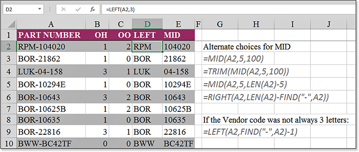
LEFT makes quick work of extracting the vendor code. Several varieties of MID or RIGHT extract the part number.When a customer comes in to buy a part, he probably doesn’t care about the vendor. So the real question is, “Do you have anything in stock that can fix my problem?”
Excel offers three functions—LEFT, MID, and RIGHT—that enable you to isolate just the first or just the last characters, or even just the middle characters, from a column.
Syntax:
=LEFT(text,num_chars)
The LEFT function returns the first character or characters in a text string, based on the number of characters specified. This function takes the following arguments:
text—This is the text string that contains the characters you want to extract.num_chars—This specifies the number of characters you wantLEFTto extract.num_charsmust be greater than or equal to zero. Ifnum_charsis greater than the length of the text,LEFTreturns all thetext. Ifnum_charsis omitted, it is assumed to be1.
Syntax:
=RIGHT(text,num_chars)
The RIGHT function returns the last character or characters in a text string, based on the number of characters specified. This function takes the following arguments:
text—This is the text string that contains the characters you want to extract.num_chars—This specifies the number of characters you wantRIGHTto extract.num_charsmust be greater than or equal to zero. Ifnum_charsis greater than the length of text,RIGHTreturns all oftext. Ifnum_charsis omitted, it is assumed to be1.
Syntax:
=MID(text,start_num,num_chars)
MID returns a specific number of characters from a text string, starting at the position specified, based on the number of characters specified. This function takes the following arguments:
text—This is the text string that contains the characters you want to extract.start_num—This is the position of the first character you want to extract in the text. The first character in the text hasstart_num 1, and so on. Ifstart_numis greater than the length of the text,MIDreturns""(that is, empty text). Ifstart_numis less than the length of the text, butstart_numplusnum_charsexceeds the length of the text,MIDreturns the characters up to the end of the text. Ifstart_numis less than1,MIDreturns a#VALUE!error.num_chars—This specifies the number of characters you wantMIDto return from the text. Ifnum_charsis negative,MIDreturns a#VALUE!error.
In Figure 8.34, it is easy to extract the three-character vendor code by using =LEFT(A2,3). It is a bit more difficult to extract the part number. As you scan through the values in column A, it is clear that the vendor code is consistently three letters. With the dash in the fourth character of the text, it means that the part number starts in the fifth position. If you are using MID, you, therefore, use 5 as the start_num argument.
However, there are a few thousand part numbers in the data set. Right up front, in cell A4, is a part number that breaks the rule. LUK-04-158 contains six characters after the first dash. This might seem to be an isolated incident, but in row 10, BWW-BC42TF also contains six characters after the dash. Because this type of thing happens in real life, two errors in the first nine records are enough to warrant a little extra attention. The four possible strategies for extracting the part number are listed in G2:G6. They are as follows:
Ask
MIDto start at the fifth character and return a large enough number of characters to handle any possible length (that is,=MID(A2,5,100)).Ask
MIDto start at the fifth character but useTRIMaround the whole function to prevent any trailing spaces from being included (that is,=TRIM(MID(A2,5,100))).Ask
MIDto start at the fifth character, but calculate the exact number of characters by using theLENfunction (that is,=MID(A2,5,LEN(A2)-4)).Skip
MIDaltogether and askRIGHTto return all the characters after the first dash. This requires you to use theFINDfunction to locate the first dash—that is,=RIGHT(A2,LEN(A2)-FIND("-",A2)).
Using LEN to Find the Number of Characters in a Text Cell
It seems pretty obscure, but you will find the LEN function amazingly useful. The LEN function determines the length of characters in a cell, including any leading or trailing spaces.
Syntax:
=LEN(text)
The LEN function returns the number of characters in a text string. The argument text is the text whose length you want to find. Spaces count as characters.
There are instances in which you can use LEN along with LEFT, MID, or RIGHT to isolate a portion of text.
You can also use LEN to find records that are longer than a certain limit. Suppose you are about to order nameplates for company employees. Each nameplate can accommodate 15 characters. In Figure 8.35, you add the LEN function next to the names and sort by the length, in descending order. Any problem names appear at the top of the list.
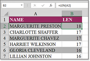
LEN identifies the number of characters in a cell.Using SEARCH or FIND to Locate Characters in a Particular Cell
Two nearly identical functions can scan through a text cell, looking for a particular character or word. Many times, you just want to know if the word appears in the text. These functions go further than telling you if the character exists in the text; they tell you at exactly which character position the character or word is found. The character position can be useful in subsequent formulas with LEFT, RIGHT, or REPLACE.
First, let’s look at an example of using FIND to determine whether a word exists in another cell. Figure 8.36 shows a database of customers. The database was created by someone who doesn’t know Excel and jammed every field into a single cell.
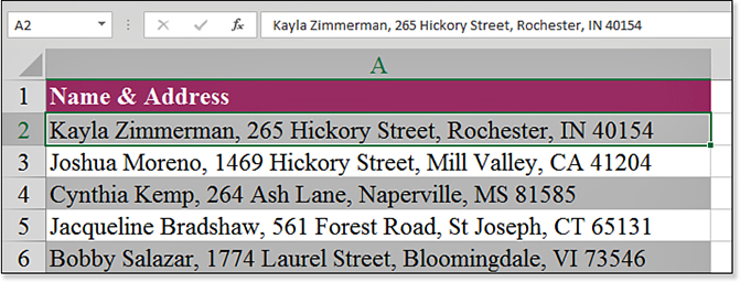
Here is how to make this work properly:
To find all the customers in California, in cell B2, enter
=FIND(", CA",A2). When you enter the formula, you get a#VALUE!error. This is okay. In fact, it is useful information: It tells you that CA is not found in the first record.Copy the formula down to all rows.
Note
Like all the other data sets in this book, these names and addresses are randomly generated from lists of the most popular first name, last name, street name, and city names. Don’t try to send Christmas cards to these people, because none of the addresses exist. And don’t think that the ZIP Codes are real; everything here is completely random.
Sort low to high by column B. You’ll see that 98% of the records have a
#VALUE!error and sort to the bottom of the list. The few California records have a valid result for the formula in column B and sort to the top of the list, as shown in Figure 8.37.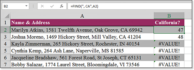
Figure 8.37 You don’t care where FINDfound the text; you simply want to divide the list into records with valid values versus errors.
FIND and SEARCH are similar to one another. The SEARCH function does not distinguish between uppercase and lowercase letters. SEARCH identifies CA, ca, Ca, and cA as matches for CA. If you need to find a cell with exactly AbCdEf, you need to use the FIND command instead of SEARCH. Also, SEARCH allows for wildcard characters in find_text. A question mark (?) finds a single character, and an asterisk (*) finds any number of characters.
The FIND function makes it easy to find the first instance of a particular character in a cell. However, if your text values contain two instances of a character, your task is a bit more difficult. In Figure 8.38, the part numbers in column A really contain three segments, each separated by a dash:
To find the first dash, enter
=FIND("-",A2)in column B.Caution
The trick with this application of
FINDis to look for something that is likely to be found only in California records. If you had customers in Cairo, Illinois, they would have also been found by theFINDcommand you just used. The theory with this sort of search is that you can quickly check through the few matching records to find false positives.To find the second dash, use the optional
start_numparameter to theFINDfunction. Thestart_numparameter is a character position. You want the function to start looking after the first instance of a dash. This can be calculated as the result of the firstFINDin column B plus one. Thus, the formula in cell C2 is=FIND("-",A2,B2+1).After you find the character positions of the dashes, isolate the various portions of the part number. In column D, for the first part of the number, enter
=LEFT(A2,B2–1). This basically asks for the left characters from the part number, stopping at one fewer than the first dash.In column E, for the middle part of the number, enter
=MID(A2,B2+1,C2–B2–1). This asks Excel to start at the character position one after the first dash and then continue for a length that is one fewer than the first dash subtracted from the second dash.In column F, for the final part of the number, enter
=RIGHT(A2,LEN(A2)–C2). This calculates the total length of the part number, subtracts the position of the second dash, and returns those right characters.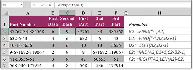
Figure 8.38 Formulaically isolating data between the first and second dashes can be done, but it helps to break each number down into small parts.
Syntax:
=FIND(find_text,within_text,start_num)
FIND finds one text string (find_text) within another text string (within_text) and returns the number of the starting position of find_text from the first character of within_text. You can also use SEARCH to find one text string within another, but unlike SEARCH, FIND is case sensitive and doesn’t allow wildcard characters.
The FIND function takes the following arguments:
find_text—This is the text you want to find. Iffind_textis""(that is, empty text),FINDmatches the first character in the search string (that is, the character numberedstart_numor1).find_textcannot contain wildcard characters.within_text—This is the text that contains the text you want to find.start_num—This specifies the character at which to start the search. The first character inwithin_textis character number 1. If you omitstart_num, it is assumed to be 1.
Syntax:
=SEARCH(find_text,within_text,start_num)
SEARCH returns the number of the character at which a specific character or text string is first found, beginning with start_num. You use SEARCH to determine the location of a character or text string within another text string so that you can use the MID or REPLACE function to change the text.
The SEARCH function takes the following arguments:
find_text—This is the text you want to find. You can use the wildcard characters question mark (?) and asterisk (*) infind_text. A question mark matches any single character; an asterisk matches any sequence of characters. If you want to find an actual question mark or asterisk, you type a tilde (~) before the character. If you want to find a tilde, you type two tildes. Iffind_textis not found, a#VALUE!error is returned.within_text—This is the text in which you want to search forfind_text.start_num—This is the character number inwithin_textat which you want to start searching. Ifstart_numis omitted, it is assumed to be 1. Ifstart_numis not greater than zero or is greater than the length ofwithin_text, a#VALUE!error is returned.Caution
If
find_textdoes not appear inwithin_text,FINDreturns a#VALUE!error. Ifstart_numis not greater than zero,FINDreturns a#VALUE!error. Ifstart_numis greater than the length ofwithin_text,FINDreturns a#VALUE!error.
Using SUBSTITUTE to Replace Characters
When you have the capability to find text, you might want to replace text. Excel offers two functions for this: SUBSTITUTE and REPLACE. The SUBSTITUTE function is easier to use and should be your first approach.
Syntax:
=SUBSTITUTE(text,old_text,new_text,instance_num)
The SUBSTITUTE function substitutes new_text for old_text in a text string. You use SUBSTITUTE when you want to replace specific text in a text string; you use REPLACE when you want to replace any text that occurs in a specific location in a text string.
The SUBSTITUTE function takes the following arguments:
text—This is the text or the reference to a cell that contains text for which you want to substitute characters.old_text—This is the text you want to replace.new_text—This is the text you want to replaceold_textwith.instance_num—This specifies which occurrence ofold_textyou want to replace withnew_text. If you specifyinstance_num, only that instance ofold_textis replaced. Otherwise, every occurrence ofold_textin text is changed tonew_text.
Using REPT to Repeat Text Multiple Times
The REPT function repeats a character or some text a certain number of times.
Syntax:
=REPT(text,number_times)
The REPT function repeats text a given number of times. You use REPT to fill a cell with a number of instances of a text string. This function takes the following arguments:
text—This is the text you want to repeat.number_times—This is a positive number that specifies the number of times to repeat text. Ifnumber_timesis0,REPTreturns""(that is, empty text). Ifnumber_timesis not an integer, it is truncated. The result of theREPTfunction cannot be longer than 32,767 characters.
In Microsoft Word, it is easy to create a row of periods between text and a page number. In Excel, you have to resort to clever use of the REPT function to do this.
In Figure 8.39, column A contains a page number. Column B contains a chapter title. The goal in column C is to join enough periods between columns B and A to make all the page numbers line up.
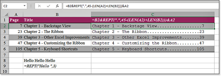
REPT function can be used to calculate a certain number of repeated entries.The number of periods to print is the total desired length, less the length of columns A and B. The formula for cell C2 is =B2&REPT(".",45-(LEN(A2)+LEN(B2)))&A2.
Note
To make this work, you must change the font in column C to be a fixed-width font, such as Courier New.
Tip
An alternative solution is to format column A with the custom format of "@*.". This shows the text in the cell and follows it with a series of periods, enough to fill the current width of the column.
Using EXACT to Test Case
For the most part, Excel isn’t concerned about the case. To Excel, ABC and abc are the same things. In Figure 8.40, cells A1 and B1 contain the same letters, but the capitalization is different.
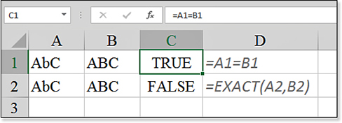
EXACT to find out whether they are equal and the same case.The formula in cell C1 tests whether these values are equal. In the rules of Excel, AbC and ABC are equivalent. The formula in cell C1 indicates that the values are equal. To some people, these two text cells might not be equivalent. If you work in a store that sells the big plastic letters that go on theater marquees, your order for 20 letter a figures should not be filled with 20 letter A figures.
Excel forces you to use the EXACT function to compare these two cells to learn that they are not the same.
Syntax:
=EXACT(text1,text2)
The EXACT function compares two text strings and returns TRUE if they are the same and FALSE otherwise. EXACT is case sensitive but ignores formatting differences. You use EXACT to test text being entered into a document. This function takes the following arguments:
text1—This is the first text string.text2—This is the second text string.
Using TEXT to Format a Number as Text
Excel is great at numbers. Put a number in a cell, and you can format it in a variety of ways. However, when you join a cell containing text with a cell containing a number or a date, Excel falls apart.
Consider Figure 8.41. Cell A11 contains a date and is formatted as a date. When you join the name in cell B11 with the date in cell A11, Excel automatically converts the date back to a numeric serial number. This is frustrating.
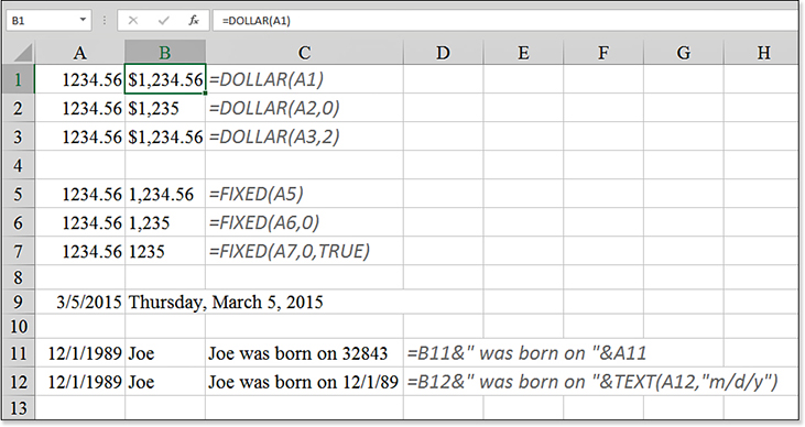
TEXT can be used to format a number as text.Today, the TEXT function is the most versatile solution to this problem. If you understand the basics of custom numeric formatting codes, you can easily use TEXT to format a date or a number in any conceivable format. For example, the formula in cell C12 uses =TEXT(A12,"m/d/y") to force the date to display as a date.
The TEXT function gives you a lot of versatility. To learn the custom formatting codes for a cell, you can select the cell, display the Format Cells dialog box (by pressing Ctrl+1), and select the Custom category on the Number tab. Excel shows you the codes used to create that format.
If you don’t care to learn the number formatting codes, you can use either the DOLLAR or FIXED function to return a number as text, with a few choices regarding the number of decimals and whether Excel should use the thousands separator. The formulas shown in C1:C7 in Figure 8.41 return the formatted text values shown in column B.
Syntax:
=TEXT(value,format_text)
The TEXT function converts a value to text in a specific number format. Formatting a cell with an option on the Number tab of the Format Cells dialog box changes only the format, not the value. Using the TEXT function converts a value to formatted text, and the result is no longer calculated as a number.
The TEXT function takes the following arguments:
value—This is a numeric value, a formula that evaluates to a numeric value, or a reference to a cell that contains a numeric value.format_text—This is a number format in text form from the Category box on the Number tab in the Format Cells dialog box.format_textcannot contain an asterisk (*) and cannot be the general number format.
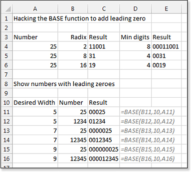
Using the T and VALUE Functions
The T and VALUE functions are left over from Lotus days.
=T("text") returns the original text. If cell B1 contains the number 123, =T(B1) will return empty text. Basically, T() returns the value in the cell only if it is text.
=VALUE() converts text that looks like a number or a date to the number or the date.