
Chapter 14
Summarizing Data Using Subtotals or Filter
Subtotaling Daily Dates by Month
Using the Advanced Filter Command
Excel in Practice: Using Formulas for Advanced Filter Criteria
The Subtotal command was added way back in Excel 97. Not enough people realize that the command is in Excel, and those who have tried it often don’t realize how powerful the command truly is. I used to have a regular gig as the Excel guy on Leo Laporte’s Call for Help television show. During one appearance, I showed people how to use the Subtotal command. I figured it was probably the most boring six minutes of television in the history of the world. However, that one show generated more fan email than any other. People wrote to say that they had been spending two hours every day adding subtotals manually, and now they used the trick from the show to reduce the task to a minute.
Filtering enables you to quickly wade through waves of data and see only the records needed to answer an ad-hoc query. Excel continues to improve the AutoFilter feature with hopes that you will never have to venture into the complicated Advanced Filter feature. When it’s combined with the Remove Duplicates command, you might never have to use the Advanced Filter.
The elusive Filter by Selection feature enables you to invoke filters even faster than before.
Duplicate data is a common problem in Excel. Beginning with Excel 2007, Microsoft provided tools to make finding and eliminating duplicates easier.
Adding Automatic Subtotals
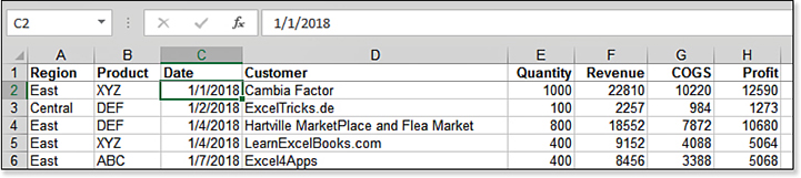
When you have a database of detailed data, you might want to add subtotals to each group of records. If your data has one field that identifies the groups, you can use the Subtotals command to add the subtotals quickly. Figure 14.1 shows a data set that is suitable for this.
Follow these steps to add subtotals to a data set:
Sort the data set by your group field. Select one cell in that column and then select Data, Sort & Filter, AZ.
Select one cell in your data set.
Select Data, Outline, Subtotal. Excel displays the Subtotal dialog box.
In the Subtotal dialog box, change the At Each Change In drop-down menu to reflect your group field.
Ensure that Use Function is set to Sum.
For each field you want to be totaled, select the field in the Add Subtotal To list, as shown in Figure 14.2.
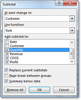
Figure 14.2 You specify the fields to be totaled in the Subtotal dialog box. If you want a page break after each group, select Page Break Between Groups.
Click OK to add subtotals. Excel adds a subtotal between each group, as shown in Figure 14.3.
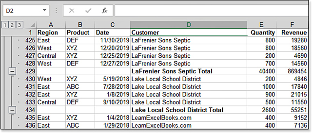
Figure 14.3 Excel inserts extra rows between groups and adds subtotals.
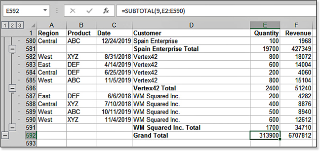
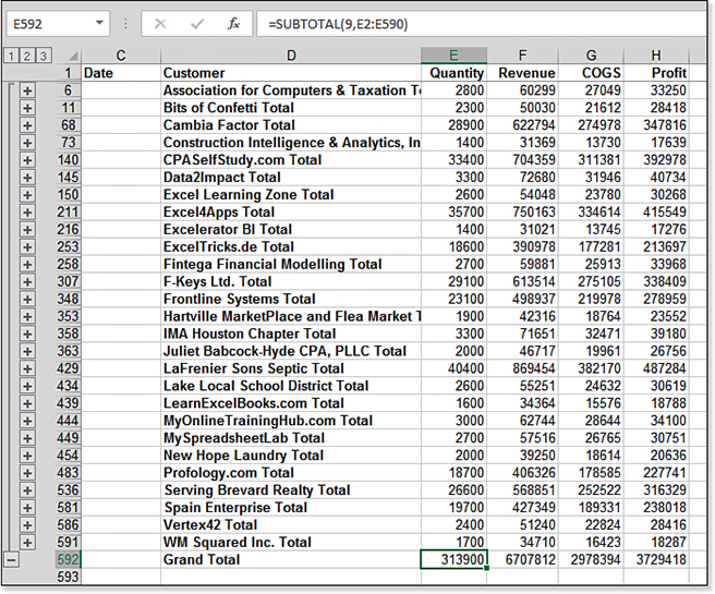
At the very bottom of the data set, Excel has added a Grand Total row. This row is smart enough to ignore all the other subtotal rows in the data set (see Figure 14.4).
Adding hundreds of subtotal rows is amazing in and of itself. However, the subtotals command offers so much more. You can go on to show only the subtotals, show the largest groups at the top, or copy the subtotals.
Working with the Subtotals
Take a close look at the left side of the worksheet in Figure 14.3. You see three new buttons to the left of column A labeled 1, 2, and 3. Those buttons are called Group and Outline buttons and were added automatically by the Subtotals command. They are the key to further analysis of the subtotals.
Showing a One-Page Summary with Only the Subtotals
Click the #2 button that appears to the left of and just above cell A1. Excel hides all the detail rows, leaving only the customer subtotals and the Grand Total row.
After setting the print area, you would have a one-page summary of the 500+ rows of data (see Figure 14.5).
If you click the #1 Group and Outline button, Excel hides everything except for the Grand Total. If you click the #3 button, Excel brings the detail rows back.
Sorting the Collapsed Subtotal View with the Largest Customers at Top
In Figure 14.5, you have the customers in alphabetical sequence. However, your manager is probably going to want to see the largest customers at the top of the report.
Think about this request, though. In row 211, the subtotal for Excel4Apps is one of the largest customers in the group, adding up data in rows 151 through 210. If you try to sort in descending order, and the data in row 211 comes up to row 3, the formula that looks at 60 rows of data will certainly evaluate to a #REF! error.
Amazingly, though, you can easily sort data when it is in the collapsed #2 view. Follow these steps:
Add subtotals as described earlier in this chapter.
Collapse the subtotals by clicking the #2 Group and Outline button.
Select one single cell in your revenue column.
Sort in descending order by clicking the ZA button on the Data tab.
The result is shown in Figure 14.6. The total for Excel4Apps flies out near the top of the data set, but it does not come to row 3. Instead, the total comes to row 128. The total for the largest customer is in row 67.
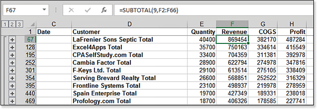
Figure 14.7 shows the #3 view of Figure 14.6. You can see that Excel sorted groups of records when the data was collapsed. All the detail rows for a customer come along with the subtotal row, but the detail rows are not sorted by revenue.

Copying Only the Subtotal Rows
A problem occurs when you try to copy the collapsed subtotal rows from Figure 14.6. If you select D1:H592, Copy, and then Paste the data to a new worksheet, you discover that Excel has copied all the hidden rows as well. Worse, the pasted data no longer has the group and outline symbols, so there is no way to collapse the data again.
The key to this task is to use a trick called Go To Special, Visible Cells Only. Excel still makes it hard to find this command.
Follow these steps:
Add subtotals to a data set as described previously.
Collapse to the subtotal-only view by clicking the #2 Group and Outline button.
Select the entire range of collapsed subtotals.
Open the Find and Select drop-down menu from the right side of the Home tab. Select the Go To Special command. Excel displays the Go To Special dialog box, as shown in Figure 14.8. This dialog box enables you to narrow a selection to only certain types of elements within your selection. This is a powerful dialog box.
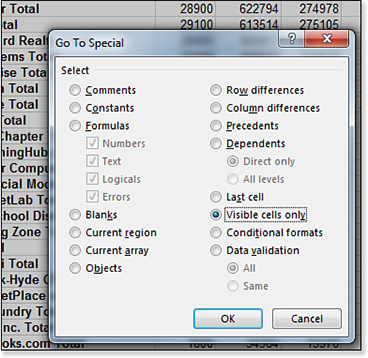
Figure 14.8 The Go To Special dialog box enables you to reduce your selection to items meeting certain criteria. In the Go To Special dialog box, select Visible Cells Only. Click OK. Excel deselects all the hidden rows.
Tip
You can replace steps 4 and 5 with a single keystroke. Hold down the Alt key while pressing the semicolon key. It turns out that Alt+; is the equivalent of selecting Home, Find & Select, Go To Special, Visible Cells Only, OK. Or, if you prefer to use the mouse, customize the Quick Access Toolbar (QAT) with an icon called Select Visible Cells.
Click Ctrl+C to copy those rows. As you can see in Figure 14.9, Excel has selected each visible row separately.
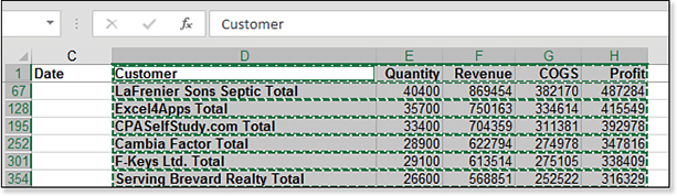
Figure 14.9 Excel copies only the visible rows. Select a blank section of the workbook. Use Ctrl+V to paste only the subtotals. The subtotal formulas are converted to values. This is the only thing that would make sense.
Formatting the Subtotal Rows
When the Subtotal command adds subtotals, it inserts a new row for each subtotal. Excel copies your key field to the new row and appends the word Total after the key field. This text in the key field column appears in bold font. Unfortunately, Excel does not widen this column, so frequently the word Total appears to be truncated because it will not fit in the column.
The other subtotal columns get a formula that uses the SUBTOTAL function. Strangely, the cells containing the formulas in each subtotal row are not bold.
When I am doing my Power Excel seminars, I’m frequently asked how to bold the subtotal rows. Many people will try selecting E67:H592 in the collapsed #2 view and pressing Ctrl+B. Although this initially looks like it works, it actually fails.
The problem becomes apparent when you go back to the #3 view to see the detail rows. The detail rows up through row 66 are fine. The problem is that all the detail rows from row 68 through the end of the data set have been bolded. For some reason, Microsoft formats the rows that are hidden as a result of the Subtotal command.
At this point, many people press Undo twice and start the process of manually formatting each subtotal row. There is, of course, an easier way. Follow these steps to format the subtotal rows:
Add subtotals to a data set as described previously.
Click the #2 Group and Outline button to collapse the data set to show only the subtotals.
Select from the first subtotal row down to the grand total row. In the current data set, select from D67 through H592.
Hold down Alt and press semicolon. Excel selects on the visible rows, which in this case are only the subtotal rows.
Apply any desired formatting. In Figure 14.10, the cells are showing a mix of Cell Styles, Heading 4, and a light red background from the Fill drop-down menu.
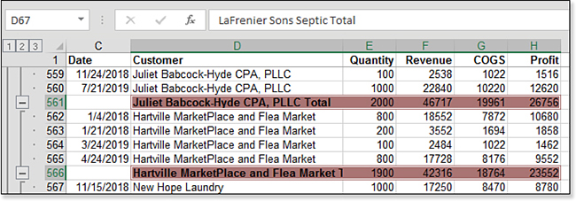
Figure 14.10 Format only the subtotal rows. Click the #3 Group and Outline button to show all the detail rows.
Step 4 in this process is the key step. Using Alt+; selects only the visible rows in the collapsed subtotal view.
Removing Subtotals
After you add subtotals and copy those subtotal rows to another worksheet, you might want to remove the subtotals from the original data set. Follow these steps to remove the subtotals:
Select one cell in the subtotaled data set.
Go back to the Subtotals command on the Data tab of the ribbon.
In the lower-left corner of the Subtotals dialog box, click the button for Remove All.
The subtotal rows are removed.
Subtotaling Multiple Fields
Suppose you want to add subtotals by region and product. You will add the subtotals twice. In the second Subtotal command, make sure you clear the Replace Current Subtotals check box.
Make sure that your data is sorted properly. You can either use the Sort dialog box to sort by region and then by product, or you can follow this set of steps, which requires only four clicks:
Select one cell in the Product column.
Click the AZ button on the Data tab.
Select one cell in the Region column.
Click the AZ button on the Data tab.
Because the sort in step 4 keeps the ties in the previous sequence, this set of steps effectively sorts by product within the region.
It is important that you add subtotals to the outer group first. Use the instructions earlier in this chapter in the “Adding Automatic Subtotals” section to add totals to the Region field.
Run the Subtotals command again. This time, specify Each Change In Product. Clear the Replace Current Subtotals check box.
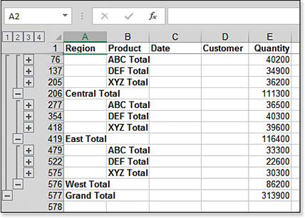
You now have four Group and Outline buttons. If you press the #3 button, you see product totals and region totals, as shown in Figure 14.11. Note that Excel supports a maximum of eight Group and Outline buttons so that you could add up to six levels of subtotals.
Subtotaling Daily Dates by Month
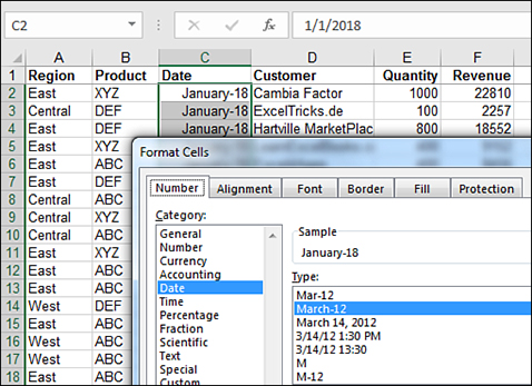
Say that you have daily dates and want to apply the subtotal after each month. Sort your data by the data field. Select the data column and apply a format that shows month and year as shown in Figure 14.12.
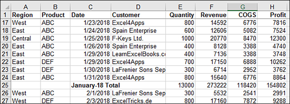
Add the Subtotals for each change in Date. The subtotals will appear after each month. You can change the format for the date column back to a short date. The result, as shown in Figure 14.13, is daily dates with monthly subtotals.
Filtering Records
The feature formerly known as AutoFilter is now called Filter. Along with the new name, the command has new features. Filtering works on any range of data with headings in the first row of the range. It works with ranges that have been defined as tables as well as regular ranges.
If you haven’t visited the Filter since Excel 2003, the following features are new:
The Search box enables you to search for values that match a wildcard. You can add the search results to a previous filter. Thus, you could quickly find all records that contain “bank” or “credit union.”
Multiselection is available in the Filter drop-down menu. If you need to select two, three, or ten values from the filter, it is easy to do now. On the flip side, it is slightly more difficult to filter to a single value because you first must uncheck the (Select All) box.
You can filter by color or icon set.
You can filter text columns based on cells that begin with a value, end with a value, or contain a value.
You can filter number columns based on cells that are greater than, less than, or between values. You can choose Top 10, Above Average, or Below Average.
You can filter date values by year or month. You can filter to conceptual values such as This Month, Last Quarter, or Year To Date.
You can filter by selection. Rather than choosing from the Filter drop-down menu, you can select any value and use Filter By Selection to filter the data to that value.
The various features work great when one column contains values of the same type. For example, Excel expects that if you have dates in a column, all the cells except the header will be dates. Excel offers special text, number, or date formats based on what it sees in the column.
Using a Filter
The icon to turn on the filter drop-down menus toggles the feature on and off. To turn on the feature, click the icon once. To turn off the feature, click the icon again. You must select one cell in your data range before clicking the filter. You should have no blank rows or blank columns in the range to be filtered.
You can turn on the filter drop-down menus by using any of these methods:
From the Data tab, select Filter.
From the Home tab, open the Sort & Filter drop-down menu and choose Filter.
Apply a table format to a range.
Right-click any cell, select Filter, and then select one of the options under Filter. In addition to performing the filter, this will turn on the Filter feature if it was not previously turned on.
Choose any value and then select the AutoFilter icon from the QAT. The Filter by Selection feature has been in Excel since Excel 2003, but the icon has never been included in the standard user interface. Also, this icon has always been mislabeled in the Customize dialog box. See “Filtering by Selection—Easy Way,” later in this chapter, for more information.
When the filter is turned on, a drop-down menu arrow is added to each heading in the range.
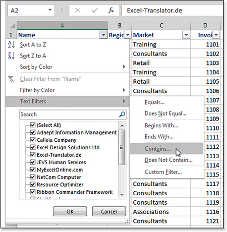
Figure 14.14 shows the menu available for one drop-down menu. This particular column includes text values, so the special filter fly-out menu includes various special text filters.
Selecting One or Multiple Items from the Filter Drop-Down
In legacy versions of Excel, the filter drop-down menu included a simple list of items in the column, and you selected one of the values. The multiselect nature of filters included since Excel 2007 offers far more power, but you have to exercise special care in using the drop-down menu.
Follow these steps to select a single item:
When you initially select the drop-down menu, all the check boxes that appear in the column are selected, as shown in Figure 14.14.
To select a single value, click Select All. This clears all the items in the list, as shown in Figure 14.15.
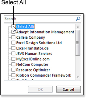
Figure 14.15 Click Select All to clear the check boxes for all items. Click the value on which you want to filter, as shown in Figure 14.16.
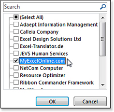
Figure 14.16 When the check boxes have been cleared, select the one value of interest and click OK. Click OK at the bottom of the drop-down menu to apply the filter.
The process you use to filter to multiple values is similar. First, click Select All to clear the check boxes for all items. You can then select the items that should be included in the filter.
Tip
With more than 1 million rows in Excel, you have the possibility for a long list of items in the Filter list—up to 10,000 items. Using the scrollbar to navigate through a list of 10,000 items will be inexact. However, there is a fast way to jump to a certain section of the list. Click any name in the list to activate the list. Then, type the first letter of your selection. Excel instantly jumps to the first item that starts with this letter. You can then use the PgDn or PgUp keys to move quickly through the items that start with that letter.
The multiselection capability is a vast improvement for filtering that can be completed in four clicks. Even though the old AutoFilter in legacy versions of Excel required only two clicks, the improvements are worth this hassle. For example, when you need to select everything except one certain value, you select the drop-down menu, clear the undesired value, and click OK.
Identifying Which Columns Have Filters Applied
Listed here are the visual clues in Excel 2019 you can use to identify columns in which a filter has been applied to a data set:
The row numbers in the range appear in blue to indicate that the rows have a filter applied.
The message area of the status bar in the lower-left corner of the screen shows a message similar to “2 of 34 records found.”
The drop-down menu for the filtered column changes from a simple drop-down menu arrow to a Filter icon, as shown in Figure 14.17.
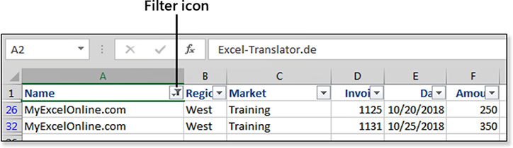
Figure 14.17 After you apply a filter to column A, the icon on the filter drop-down menu changes.
Combining Filters
Filters are additive, which means that after you place a filter on a column, you can apply a filter to another column to show even fewer rows. You can apply two filters to the same column, such as when you want to select all the West region cells that are red.
Clearing Filters
After you apply a filter, you have several options for clearing it:
From the filter drop-down menu, select Clear Filter from Column. This leaves filters on in other columns.
From the filter drop-down menu, choose a different filter.
From the Data tab, select Clear from the Sort & Filter group. This clears selected filters from any column but leaves the drop-down menus in place, so you can continue to select other filters.
Select the Filter icon from the Data tab or the Home tab to clear all filters and turn off the filter feature.
Refreshing Filters
Keep in mind that when data in a range changes, the filters do not update automatically. This can happen when you add new rows or edit data. It can also happen if your data range has formulas that point to lookup tables in other parts of the workbook. In such a case, you need to have Excel calculate the filter again. Excel calls this feature Reapply. There are several ways you can reapply a filter:
On the Data tab, select the Reapply icon.
On the Home tab, select Sort & Filter, Reapply.
Right-click a cell and then select Filter, Reapply.
Resizing the Filter Drop-Down
The filter drop-down menu always starts fairly small. If you have a long list of items, you might want the drop-down menu to be larger. To do this, hover your mouse over the three dots in the lower-right corner of the drop-down menu. When the mouse pointer changes to a two-headed diagonal arrow, click and drag down or to the right.
Filtering by Selection—Hard Way
You can filter without using the filter drop-down menus. Microsoft Access has offered a Filter by Selection icon in the toolbar for more than a decade. Excel includes this functionality, but it is hidden where most people will never find it.
To access the Filter by Selection feature, right-click any cell and then select Filter from the context menu. You then have an opportunity to filter based on the cell’s value, color, font color, or icon, as shown in Figure 14.18.
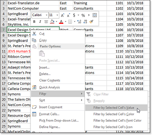
The Filter by Selection feature works even if the filter drop-down menus have not been activated previously. Using this feature turns on the filter drop-down menus for the data set.
It would be helpful if you could use this feature to select multiple values, such as selecting a cell that says East and then Ctrl+clicking a cell for West. You might think that filtering by selection would filter to both East and West, but that does not work in Excel 2019.
Filtering by Selection—Easy Way
The fast way to filter by selection is to add the AutoFilter icon to the Quick Access Toolbar.
To get one-click access to Filter by Selection, follow these steps:
Right-click the Quick Access Toolbar and select Customize Quick Access Toolbar.
In the Choose Commands From Drop-Down menu, select Commands Not In The Ribbon.
In the left list box, browse to and select AutoFilter, as shown in Figure 14.19. Click the Add button.
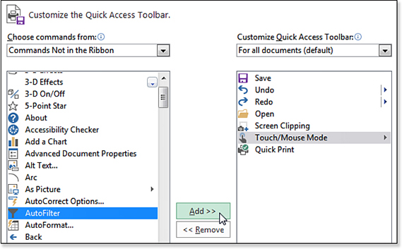
Figure 14.19 The icon labeled “AutoFilter” actually is Filter By Selection. Click OK to close the Excel Options dialog box.
To use Filter by Selection, select a value in one of the data rows. Click the AutoFilter icon in the Quick Access Toolbar. If the data set did not previously have the filter drop-down menus, Excel turns on the Filter feature and filters the data set based on the value in the active cell.
Filter by Selection is additive, which means you can choose another value in another column and click the AutoFilter icon to filter the data set further.
In Figure 14.20, the data set is filtered to show Central region invoices for the Consultants market. This was accomplished in four mouse clicks:
Select a cell that contains Central, such as B4.
Click the AutoFilter icon in the Quick Access Toolbar.
Select Consultants in cell C17.
Click the AutoFilter icon.
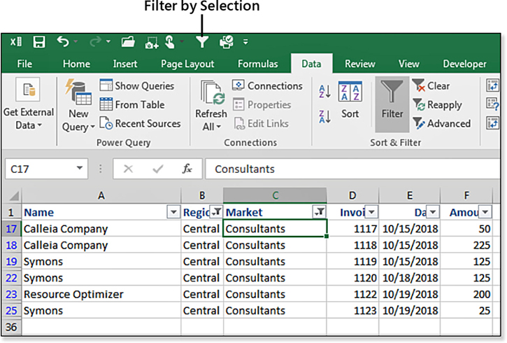
Figure 14.20 Filter by Selection is used twice to filter based on column C and then on column B.
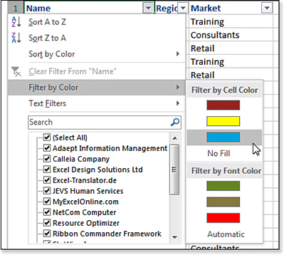
Filtering by Color or Icon
The improved Conditional Formatting commands give you many ways to change the color of a cell. Filter by Color is a great way to find all of the records that match a color applied either through conditional formatting or the fill color or font color drop-down menu menus.
Imagine that you are tracking numerous projects in Excel. You manually highlight certain projects in red if you are missing key elements of the project information. You can use Filter by Color to show only the rows that have a red fill.
Filter by Color works for the cell color, font color, or the icon in the cell.
As shown in Figure 14.21, the Filter by Color fly-out menu offers to filter based on fill color, font color, or icon. Note that the sections of the fly-out menu appear only if you have used color or icons in the range. If all your cells contain black text, Filter by Font Color will not appear in the fly-out menu. If your range contains all black text on a white background, without icons, the Filter by Color menu will be disabled.
Handling Date Filters
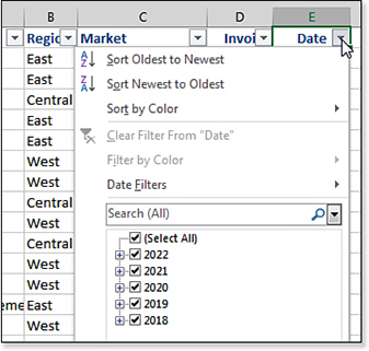
The filter drop-down menu for date columns automatically groups the dates into hierarchical groups.
In Figure 14.22, the underlying data contains daily dates. However, the default drop-down menu shows options for the years found in the data set.
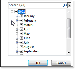
Click the plus sign next to any year to expand the list to show months within the year, as shown in Figure 14.23. You can then click the plus sign next to a month to see the days within the month.
Troubleshooting
You might hate the grouping of dates in the Filter menu. If your data set includes only a few scattered dates such as February 2, May 30, July 4, and September 4, wading through the grouped filters is annoying.
You can turn off the hierarchical grouping of dates in the filter drop-down menu. To do so, click the File menu and choose Options. In the Options dialog box, choose the Advanced category. Scroll down to the section for Display For This Workbook. Next, select a workbook, and then clear the check box for Group Dates in the AutoFilter Menu.
Using Special Filters for Dates, Text, and Numbers
Excel examines the data in a column to determine whether it contains mostly text, dates, or numeric values. Depending on which data type appears most often, Excel offers special filters designed for that data type.
For columns that contain mostly text, Excel offers the filters Begins With, Ends With, Contains, Does Not Contain, Equals, and Does Not Equal. You are allowed to use wildcard characters in these filters. For example, you can use an asterisk (*) for any number of characters or a question mark (?) to represent a single character. The Contains filter seems obsolete with the Search box in the Filter drop-down menu.
For columns with mostly numeric values, the special filters include Top 10, Above Average, Below Average, Between, Less Than, Greater Than, Does Not Equal, and Equals. For the Top 10 filter, you can specify the top or bottom values. You can also specify whether the results are based on the top 10 items or the top 10 percent of items. Finally, you can change the number 10 to any number. Thus, you can use this filter to show the bottom 20 percent or the top three items.
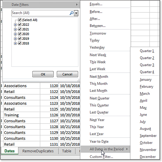
For columns with mostly dates, the special filters include Before, After, or Between a particular day, week, month, quarter, or year. The special filters also include Year To Date or All Dates In The Period, as shown in Figure 14.24.
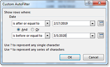
All the special filters offer a pathway to the legacy Custom AutoFilter dialog box. This filter enables you to combine two conditions by using an AND or OR clause. This feature solves your problems some of the time, but there are still complex conditions that require you to resort to using the advanced filter.
The Custom AutoFilter dialog box was nominally improved in Excel 2007. For example, a calendar control was added that can be used to select dates when you are filtering a date column. You can use the dialog box shown in Figure 14.25 to select dates that are within a certain range of dates.
Totaling Filtered Results
After you have applied a filter, you might want to sum the visible cells in a column. This task is straightforward in Excel 2019. Select the first visible blank cell below the column and click the AutoSum button. Instead of inserting a SUM function, Excel inserts a SUBTOTAL function. The =SUBTOTAL(9,F2:F1874) function sums the visible rows from a data set that has been filtered. You can edit the first argument in the SUBTOTAL function to find the count, average, minimum, and maximum, as well as other calculations on the visible rows.
Formatting and Copying Filtered Results
When you apply a filter, some rows are hidden and other rows are visible. The rows hidden by the filter are different from rows hidden with the Hide Rows command. Rows that are hidden using Hide Rows are often included when you copy or format a range that contains those rows. When you have manually hidden rows, you must use Alt+; to narrow your selection to only the visible rows. It is not necessary to use Alt+; when the rows have been hidden by the Filter command. Alt+; is the shortcut for Go To Special, Visible Cells Only.
You can use this behavior to format or copy rows matching certain criteria. If you want to highlight all rows matching a criterion by changing the background color of the cell, follow these steps:
Select one cell in the unfiltered data set that matches the proper criterion.
Click the Filter by Selection icon in the Quick Access Toolbar. If you don’t have this icon available, refer to Figure 14.17 and follow the instructions there.
Select the first visible cell below the headings.
Press Ctrl+Shift+Down Arrow and then Ctrl+Shift+Right Arrow to select all the cells below the heading.
Format the cells as desired.
Select Data, Filter to remove the filter and show all rows. You will find that only the rows that were visible during the filter have the new formatting.
Using the Advanced Filter Command
The Advanced Filter command is still present in Excel 2019. Microsoft should give this feature a new name because it is remarkably powerful and does much more than filtering. However, the Advanced Filter command is admittedly one of the more confusing commands in Excel. This is particularly true because you can use the Advanced Filter in eight ways, and each method requires slightly different steps.
Tip
You can only copy filtered results to the active sheet, not to a new sheet. However, if you start on a blank sheet, you can specify that you want to filter data from another sheet and pull that data to the active sheet.
The eight ways to use the Advanced Filter are derived by multiplying 2×2×2. There are three options in the Advanced Filter dialog box, and depending on your choices for those three options, you can have possible combinations:
You can choose either Filter In Place or Copy To A New Location.
You can choose to filter with a criteria range or without any criteria.
You can choose to return all matching values or only the unique values.
In reality, there are more than eight ways to use Advanced Filter. If you choose to copy records to a new location, you can either copy all the input columns in order or specify a subset of columns and/or a new sequence of columns.
You can build a simple filter for one column. You can combine any number of filters for multiple columns. You can build incredibly complex filters, using any formula imaginable. Alternatively, you can use no criteria at all. Using no criteria is common when you are using Advanced Filter to extract unique values or when you want to use Advanced Filter to reorder the sequence of columns.
To use Advanced Filter on a data set, follow these steps:
If you are using criteria, copy one or more headings from your data set to a blank section of the worksheet. Under each heading, list the value(s) you want to be included.
If you are using an output range and want to reorder the columns or include a subset of the columns, copy the headings into the appropriate order in a blank section of the worksheet. If you want all the original columns in their original sequence, the output range can be any blank cell.
Select a cell in your data range.
Select Data, Sort & Filter, Advanced.
Verify that the list range contains your original data set.
If you are using criteria, enter the criteria range.
If you want to copy the matching records to a new location, select Copy To Another Location. This enables the reference box for Copy To. Fill in the output range.
If you want the output range to contain only unique values, click Unique Records Only. If your output range contains a single field, a list of the values in that field is displayed that match the criteria. If your output range contains two or more fields, every unique combination of those two or more fields is displayed.
Click OK to perform the filter.
Excel in Practice: Using Formulas for Advanced Filter Criteria
Sometimes you might need to filter based on criteria that are too complex for any of Excel’s built-in rules. For example, suppose you want to create an advanced filter to find all records in which one of 30 customers bought one of 20 products. The necessary criteria range would cover 601 rows and would take hours to build.
There is one obscure syntax of advanced filter criteria that enables you to filter to anything for which you can build a TRUE/FALSE formula. Use the following specifics to set up a filter that contains formulas:
This criteria range is two cells tall by one column wide.
The top cell is blank or contains text not found in the data range headers.
The second cell contains a formula that should have relative references pointing to the first data row of the input range.
The formula should evaluate to
TRUEorFALSE. For example, to select all the West records where the invoice is above average for the West, use this:=AND(B2="West",F2>AVERAGEIF($B$2:$B$1874,"West",$F$2:$F$1874))
When Excel sees that the first row of the criteria range is blank, it takes the formula in the second cell and applies it to all rows in the range. Any rows that would evaluate to TRUE are returned in the filter.
Advanced Filter Criteria
Even though it is not obvious from the instructions for using Advanced Filter, you can build advanced filter criteria that can ask for a range of values. For example, if you are using an advanced filter, it is unlikely you will want to filter to the customer with exactly $7,553 in sales. However, you might want to filter to invoices that are more than $5,000 in sales. To set up this criterion, type Sales into cell K1. In cell K2, type >5000. When you issue the Advanced Filter, Excel returns all invoices more than $5,000.
In Figure 14.26, the Advanced Filter operation extracts all East region sales in the Vehicles market. Three columns from the matching records will be copied to Columns L:N.
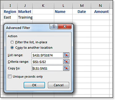
Note that criteria values that are in the same row are treated as if they were joined by AND. Because East and Vehicles are both in row 2, a record must be from the East region and have a market of vehicles to appear in the data set. If you move Vehicles from row 2 to row 3 and expand the criteria range to I1:J3, the two values are joined with an OR. All records that are from either the East region or the Vehicles market appear in the results.
Using Remove Duplicates to Find Unique Values
By its nature, transactional data has a lot of detail. You end up with transactional data in Excel because it is often the easiest to obtain. As you start to analyze transactional data, you often want to find the number of customers, number of products, or number of something in the data set.
For example, transactional data can tell you that there were 34 invoices issued last month, but that doesn’t mean there were 34 customers. Some of those customers might have made repeat purchases. In this case, 20 customers could account for 34 invoices.
To find the number of unique customers, you need a way to eliminate the duplicate records in a data set. In legacy versions of Excel, this usually meant using Advanced Filter, some IF functions, or possibly a pivot table. However, in Excel 2019, the Remove Duplicates data tool makes it easier to remove duplicates.
The first thing to realize is that the Remove Duplicates tool is destructive because it really removes the duplicate records. If you want to keep the original transactional data intact, you should either make a copy of the customer column in a blank section of the workbook or make a backup copy of the workbook.
To find the unique values in a data set, follow these steps:
Copy the data set to a blank section of the worksheet. Make sure to leave a blank column between your real data and the copy of the data.
Select a single cell within the data set.
On the Data tab, in the Data Tools group, select Remove Duplicates. Excel expands the selection to include the entire range. In the Remove Duplicates dialog box, Excel predicts if your data has headers. This dialog box also shows a list of all the fields in the data set.
Because you are interested in a unique list of customers, click the Unselect All button to clear all check boxes, and then select the Customer field, as shown in Figure 14.27.
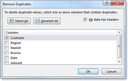
Figure 14.27 Choose which columns should be considered when analyzing duplicates. Click OK to perform the action. Excel tells you how many duplicate values were found and removed. It also tells you how many unique values remain.
Tip
Remember that the Remove Duplicates command is destructive. For this reason, sometimes you might want to find the duplicates and choose which version to remove. In that case, you Select Home, Conditional Formatting, Highlight Cell Rules, Duplicate Values.
Other times, you might want to send a copy of the unique values to a new location. In this case, use the Advanced Filter command discussed earlier in this chapter.
Finally, you might want to remove duplicates but add up the sales for all the removed records and then add them to the Customer field. Although this can be achieved with pivot tables, it can also be achieved using the Consolidate feature, which is discussed in the next section.
Combining Duplicates and Adding Values
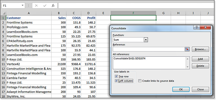
In columns A:D of Figure 14.28, each customer appears one or more times in the list with sales, cost, and profit values. In addition to finding a unique list of customers, you would like to know the total sales and profit for each customer. You can use a pivot table to find the total sales for each customer. Alternatively, you can use the data tools to consolidate the table down to one record per customer.
To use the Consolidate feature to total sales from all the records for that customer, follow these steps:
Instead of preselecting the data, move the cell pointer to a blank section of the worksheet.
Select Data, Data Tools, Consolidate. The Consolidate dialog box appears.
In the Consolidate dialog box, enter the reference to your data in the Reference box. The data will be combined based on the field in the left column of the range. If you have multiple lists of customers, you can click the Add button and enter additional ranges.
Make sure to select the Top Row and Left Column check boxes in the Use Labels In section.
Click OK.
Excel creates a new table. Each customer appears in the table just once. The sales associated with all the records of the customer appear in the new total, as shown in Figure 14.29.

Two annoyances remain with this command. First, the heading for the leftmost column is never filled in. Second, the command leaves the results in the same sequence in which they originally appeared. In this example, you will probably want to add the heading above cell F2 and sort the data.