
Chapter 16
Using Slicers and Filtering a Pivot Table
Pivot table filters have been quietly evolving over the past several versions of Excel. Excel 2010 pivot tables introduced a visual filter called a slicer. Slicers enable you to perform ad-hoc analysis by choosing various items from various fields in the pivot table. Excel 2013 added a new date-centric visual filter called a timeline.
Filtering Using the Row Label Filter
To follow along, create a new pivot table from the 16-Slicers.xlsx file. Check the Customer, Date, Quantity, Revenue, COGS, and Profit fields. On the Design tab, open the Report Layout drop-down menu. Choose Tabular form and then choose Repeat All Item Labels. Choose the Banded Rows check box on the Design tab. You will end up with the pivot table shown in Figure 16.1. Drop-down lists in cells A3 and B3 lead to the row filter menus.
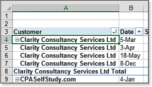
Figure 16.2 shows the Filter menu for the Customer field. This drop-down menu contains four separate filter mechanisms:
The Label Filters fly-out menu appears for fields that contain text values. You can use this fly-out to select customer names that contain certain words, begin with, end with, or fall between certain letters.
The Value Filters fly-out menu enables you to filter the customers based on values elsewhere in the pivot table. If you want only orders over $20,000, or if you want to see the Top 10 customers, use the Value Filters fly-out.
The Search box was added in Excel 2010 and is similar to using Label Filters, but faster.
The check boxes enable you to exclude individual customers, or you can clear or select all customers by using Select All.
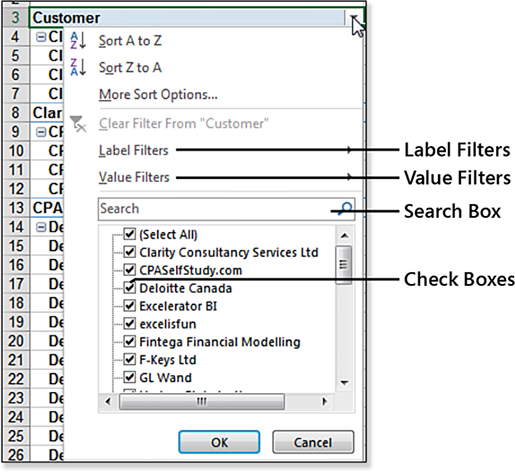
Figure 16.2 Four separate filter mechanisms exist in this drop-down menu.
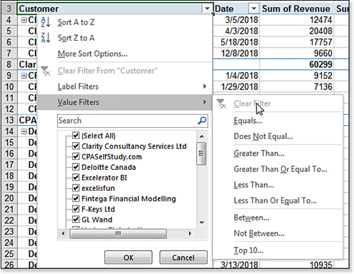
Figure 16.3 shows the detail of the Value Filters fly-out. All these filters, except Top 10, were new in Excel 2007.
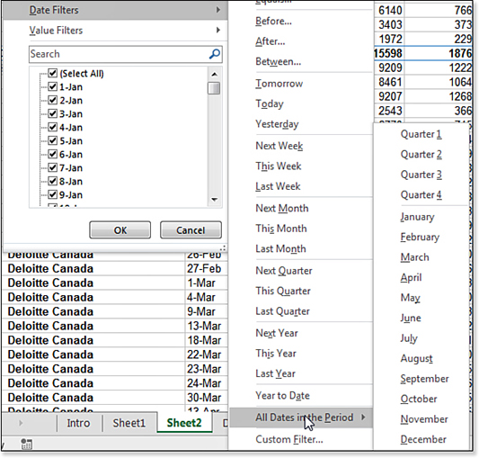
When you access the filter drop-down menu for a field that contains 100% dates, the Label Filters fly-out is replaced by a Date Filters fly-out, as shown in Figure 16.4. This fly-out offers conceptual filters, such as Last Month, Next Quarter, and This Year. The All Dates in Period choice leads to a second fly-out where you can choose based on month or quarter.
Clearing a Filter
To clear all filters in the pivot table, use the Clear icon in the Sort & Filter group of the Data tab. To clear filters from one field in the pivot table, open the filter drop-down menu for that field and select Clear Filter from “Field.”
Filtering Using the Check Boxes
The Customer drop-down menu includes a list of all the customers in the database. If you need to exclude a few specific customers, you can clear their check boxes in the filter list.
The (Select All) item restores any cleared boxes. If all the boxes are already selected, clicking (Select All) clears all the boxes.
Because it is easier to select three customers than to clear 27, if you need to remove most of the items from the list of customers, you can follow these steps:
If any customers are cleared, choose Select All to reselect all customers.
Choose Select All to clear all customers.
Select the particular customers you want to view, as shown in Figure 16.5.
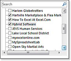
Figure 16.5 Choose Select All to clear all customers and then select the few desired customers. Troubleshooting
The Search box above the checkboxes does not get re-applied if you refresh the pivot table.
Perhaps you need to select all the customers with “Bank” in their names. You could do this with the Search box, and it would work. However, after adding more data to the source data and refreshing the pivot table, Excel will not pick up any new customers with “Bank” in their names.
A workaround is to use the Label Filters for Contains Bank. The Label Filter will be re-applied after a refresh.
Filtering Using the Label Filter Fly-Out
All the Label Filters choices shown previously in Figure 16.2 lead to the same dialog box. Suppose that you are interested in finding all customers whose name includes “Excel.” Follow these steps:
Open the Customer filter drop-down menu.
Open the Label Filters fly-out.
Select Contains. Excel displays the Label Filter dialog box.
Type
Excel. Click OK. The pivot table is filtered to customers whose name includes “Excel.”
If you open the first drop-down menu in the Label Filter dialog box, you see the following choices:
Equals
Does Not Equal
Is Greater Than
Is Greater Than Or Equal To
Is Less Than
Less Than Or Equal To
Begins With
Does Not Begin With
Ends With
Does Not End With
Contains
Does Not Contain
Is Between
Is Not Between
You can use the wildcards * and ?, with * representing any character(s) and the ? wildcard representing a single character.
Filtering Using the Date Filters
When a field in the original data set contains only values formatted as dates, Excel offers the Date Filters fly-out shown previously in Figure 16.4.
Many of the date filters contain conceptual filters. If you filter a pivot table to Yesterday and then refresh the data set a week later, the dates returned by the filter will change.
The list of conceptual filters feels like it was borrowed from QuickBooks, but it is not quite as complete as those from QuickBooks. It would be nice to have choices such as Last 30 Days, Month to Date, and so on.
The penultimate choice in the first fly-out is All Dates in the Period, which leads to a second fly-out. Choosing January or Quarter 1 is great when you have dates from several years, and you want to compare January from each year.
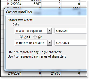
The last choice in the first fly-out is Custom Filter. As shown in Figure 16.6, you can use this filter to build a custom date range. Change the selection in the first drop-down menu to Is Between. Then use the date icons to choose your selected dates. The Whole Days check box was new in Excel 2013. Use this to truncate times from fields that contain date and time.
Filtering to the Top 10
Pivot tables offer a feature called Top 10. Despite the name, the filter is not just for finding the top 10 values. You can use the filter to find the top or bottom items. You can specify 5, 7, 10, or any number of items.
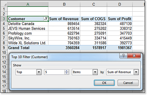
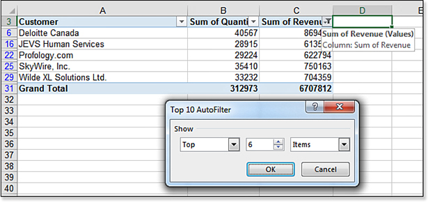
To start the filter, open the Customer filter drop-down menu. Open the Value Filters fly-out and select Top 10. Excel displays the Top 10 Filter dialog box. In Figure 16.7, the report has been filtered to show the top five customers based on revenue.
The Top 10 filter offers these options:
The first drop-down menu in the dialog box offers a choice between Top and Bottom.
The second field is a spin button and a text box. You can use the spin button to change from 5 to 10. If you need to get to 1,000,000, you should type that value into the text box instead of trying to hit the spin button 999,990 times.
The next field is a drop-down menu with choices Items, Percent, and Sum. These three choices are discussed in the next sections.
The final drop-down menu offers all the numeric fields in the VALUES area of the pivot table.
The Items/Percent/Sum drop-down menu offers a lot of flexibility. If you select Percent, the pivot table shows you enough customers so that you see n% of the value field. For example, you might ask for the top 80% of profit.
If you choose Sum, you can specify a large number as the second field in the dialog box. For example, you might want to see enough customers to reach $5 million in sales.
Filtering Using Slicers
Slicers are visual filters that make it easy to run various ad-hoc analyses. While slicers are easier to use than the Report Filter, they offer the added benefit that a slicer can filter multiple pivot tables and pivot charts created from the same data set.
Adding Slicers
To add default slicers, follow these steps:
Select one cell in your pivot table.
On the Analyze tab, select the Insert Slicer icon. Excel shows the Insert Slicers dialog box.
Choose any fields that would make suitable filter fields. In Figure 16.8, Region, Product, and Years are selected. Months, Quarters, and Date would also be effective, but you see how they can be filtered using a timeline later in this chapter. Click OK.
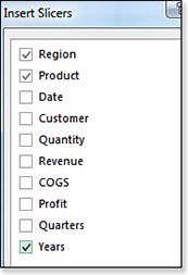
Figure 16.8 Choose all fields that are suitable for visual filters.
Excel adds default filters, tiled in the center of your screen (see Figure 16.9).
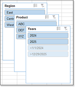
Arranging the Slicers
You can reposition and resize the slicers. Choose a logical arrangement for the slicers. Following are some examples.
The Region and Product slicers contain short entries. Make each slicer wider and then use the Columns setting in the Slicer Tools Options tab to increase each slicer to three columns. See Figure 16.10 for the setting.
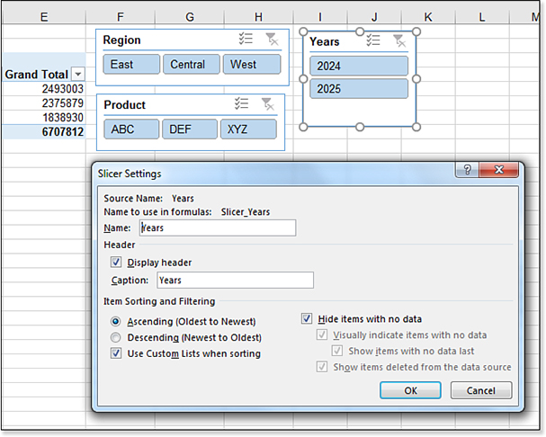
The Year slicer is wider than it needs to be. There are also two extra items (<1/1/2024 and >12/31/2025) in the slicer that are remnants of Auto Group. You can turn these off in the Slicer Settings dialog box. Select the slicer and choose Slicer Settings. Also, Hide Items with No Data is checked.
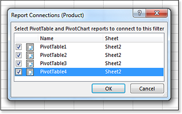
Select the slicer.
From the Slicer Tools Options tab of the ribbon, choose Report Connections.
Select each pivot table that should be filtered by the slicer.
Make sure to format both the Actuals table and the Forecast table as a table using Ctrl+T.
Rename the tables as “Actuals” and “Forecast” instead of “Table1” and “Table2.”
Copy the Region column from both tables into a new area (you don’t need the heading from the second copy).
Use Data, Remove Duplicates on the new single-column region table so each region appears once.
Format this single-column table as a table. Rename it as Regions.
Choose Data, Relationships. Add a new relationship from Region in the Actuals table to Region in the Regions table. Repeat to create a relationship from Region in the Forecast table to Region in the Regions table.
Create a Forecast pivot table. Make sure to choose Add This Data To The Data Model when creating the pivot table. Use Revenue from the Forecast table but use Region from the Regions table.
Create an Actuals pivot table following the same guidance in step 7.
When you Insert, Slicer, choose the All tab at the top of the Insert Slicer dialog. Choose to create a slicer from the Region field in the Regions table.
Using the Slicers in Excel 2019
To select a single item from a slicer, choose that item. To multiselect in Excel 2019, first, choose the icon at the top of the slicer that has the three check marks. You can now click each item. You can also use the Ctrl key to select multiple nonadjacent items or drag the mouse to select adjacent items.
Selections in one slicer might cause items in other slicers to become unavailable. In this case, those items move to the end of the list. This gives you a visual indication that the item is not available based on the current filters.
To clear a filter from a slicer, click the Funnel-X icon in the top right of the slicer.
Filtering Dates
Excel 2013 added a Timeline control for filtering date fields. It is difficult to use. Instead of the Timeline, you could achieve more flexibility by arranging three slicers for Year, Quarter, and Month, as shown in Figure 16.11
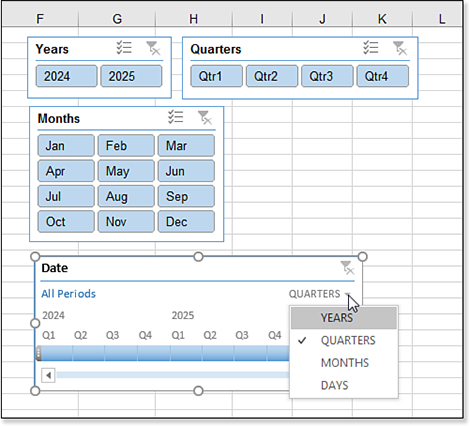
Figure 16.11 shows a timeline. The timeline has been set to filter by quarter.
Filtering Oddities
The next sections discuss a few additional features available for filtering pivot tables.
AutoFiltering a Pivot Table
I was doing a Power Excel seminar in Philadelphia when someone in the audience asked whether it is possible to AutoFilter a pivot table. The answer is no; the Filter field is not available when you are inside a pivot table.
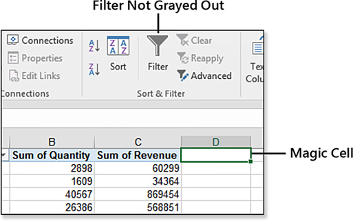
There is a surprising bug, however. If you put the cell pointer to the right of the last heading of a data set and click the Filter icon, Excel turns on the AutoFilter drop-down menus. I call this cell the magic cell.
The guy at Microsoft in charge of making the AutoFilter icon unavailable when you are in a pivot table evidently forgot about that magic cell to the right of the headings. If you put the cell pointer in cell D1 in Figure 16.12, the Filter icon remains available.
What is the advantage of using the AutoFilters? The Top 10 AutoFilter works differently from the Top 10 PivotTable filter. In Figure 16.13, the Top 10 AutoFilter for the top six items returns the top five customers and the true grand total.
If you try this method, remember that you have to go back to the magic cell to toggle off the AutoFilter. Also, if you change the underlying data and refresh the pivot table, the AutoFilter is not updated. After all, the Excel team believes that you can’t AutoFilter a pivot table.
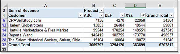
The AutoFilter lets you filter by one item along the Column field. In Figure 16.14, the report is showing the top five customers for product XYZ in column D. A regular pivot table filter would always be based on the Grand Total in column G.
Replicating a Pivot Table for Every Customer
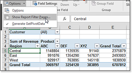
This technique makes many copies of the pivot table, with a different Report Filter value in each copy. To use the feature, you have to move the field to the FILTERS drop zone in the PivotTable Fields list. To create a report for every customer, move the Customer field to the FILTERS drop zone. Select the Options drop-down menu from the Analyze tab. Select Show Report Filter Pages from the drop-down menu, as shown in Figure 16.15. Confirm which field should be used. Excel adds worksheets to your workbook. Each worksheet contains the original pivot table, with a different value chosen for the selected filter field.
Caution
Slicers are not visible on the copied pivot tables when you use this technique.
Sorting a Pivot Table
In all the pivot tables so far in this chapter, the customers are presented in alphabetical sequence. In each case, the report would be more interesting if it were presented sorted by revenue instead of by customer name.
Starting in Excel 2010, if you use the AZ or ZA icons on the Data tab, Excel automatically sets up rules in the Sort and More Sort Options dialog boxes.
To access these settings later, open a row field drop-down menu and choose More Sort Options. This opens the Sort (Customer) dialog box. Click the More icon to access More Sort Options (Customer).