5

Leveraging DAX

Data Analysis Expressions (DAX) is a formula language that made its debut back in 2010 with the release of Power Pivot within Excel. Much of DAX is similar to Excel’s functions, and therefore, learning DAX is an easy transition for Excel users and Power users alike. In fact, DAX is so similar to Excel that we have seen new students become comfortable with the language and begin writing DAX within minutes.

The goal of this chapter is to introduce you to DAX and give you the confidence to start exploring this language on your own. Because of the limited scope of this chapter, there will not be any discussions on in-depth DAX concepts and theory. There are, of course, many other books that are dedicated to just that.

Now, let’s take a look at what is covered in this chapter:

• Building calculated columns
• Creating calculated measures
• Understanding filter context
• Working with time intelligence functions
• Role-playing tables with DAX

Now, let’s take a look at writing DAX by building calculated columns.

Building calculated columns

In this section, you will learn how to create calculated columns in Power BI using DAX. The building of calculated columns is a great way of extending the analytical capability of Power BI and by the end of this chapter, you will feel very comfortable with creating new columns through DAX. The writing of calculated columns logically occurs after the data model has been developed, therefore, in order to follow along with this section, you will need to open the pbix file Chapter 5 – Leveraging DAX.pbix from the Microsoft-Power-BI-Quick-Start-Guide-Third-EditionStarting Examples directory.

Calculated columns are stored in the table in which they are assigned, and the values are static until the data is refreshed. You will learn more about refreshing data in a later chapter.

There are many use cases for calculated columns, but the two most common are as follows:

• Adding descriptive columns
• Creating concatenated key columns

Now you are going to create your first calculated column. Before you get started though, you need to first know that Power BI Desktop provides the IntelliSense feature. IntelliSense will help you out a lot when writing code, as you will discover very soon. This built-in functionality will autocomplete your code as you go and will also help you explore and discover new functions in the DAX language. In order to take advantage of IntelliSense, you simply need to start typing in the formula bar. Now you are ready to start writing DAX!

Click on Data view—this is located on the left navigation pane of the Power BI Desktop screen. Next, click on the Customer table from the Fields list. Once the Customer table has been selected, click on New column—this is found on the Table tools ribbon, as shown in Figure 5.1:

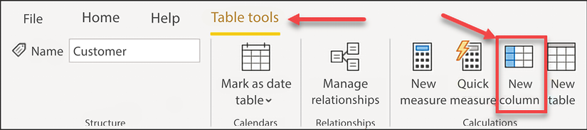
Figure 5.1: New calculated column

You will now see the text Column = in the formula bar. First, name the new column by replacing the default text of Column with Full Name. Then, move your cursor to after the equals sign and type a single quote character. Immediately after typing the single quote character, a list of autocomplete options will appear underneath the formula bar. This is IntelliSense at work. The first option in this list is the name of the table you currently have selected—Customer. Press the Tab key and the name of the table will automatically be added to the formula bar, as shown in Figure 5.2:

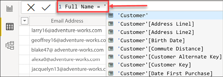
Figure 5.2: Using IntelliSense

Next, type an opening square bracket into the formula bar followed by the capital letter F, making [F. Once again, you will immediately be presented with autocomplete options. The list of options has been limited to only columns that contain the letter ƒ, and the first option available from the dropdown is First Name. Press the Tab key to autocomplete. The formula bar should now contain the following formula:

Full Name = 'Customer'[First Name]

The next step is to add a space, followed by the last name. There are two options in DAX for combining string values. The first option is the concatenate function. Unfortunately, concatenate only accepts two parameters; therefore, if you have more than two parameters, your code will require multiple concatenate function calls. On the other hand, you also have the option of using the ampersand sign (&) to combine strings.

The ampersand will first take both input parameters and convert them into strings. After this data conversion step, the two strings are then combined into one. Let’s continue with the rest of the expression. Remember to use the built-in autocomplete functionality to help you write code.

Next, add a space and the last name column. To add a space—or any string literal value for that matter—into a DAX formula, you will use quotes on both sides of the string. For example, " " inserts a space between the first and last name columns. The completed DAX formula will look like Figure 5.3:

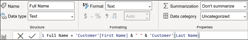
Figure 5.3: Completed DAX example for Full Name

In Figure 5.4, you see the results of the completed expression in the Customer table:

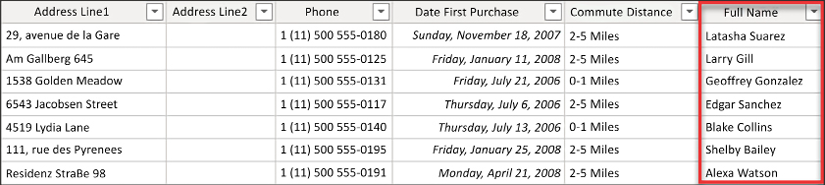
Figure 5.4: Results of the Full Name calculated column in the Customer table

Now, let’s take a look at an example of using string functions in DAX to create calculated columns.

Creating calculated columns with string functions

Now that you have completed your first calculated column, let’s build a calculated column that stores the month-year value. The goal is to return a month-year column with the two-digit month and four-digit year separated by a dash, making MM-YYYY. Let’s build this calculation incrementally.

Select the Date (Order) table and then click on New column from the Table tools ribbon. Write the following code in the formula bar and then hit Enter:

Month Year = 'Date (Order)'[Month Number of Year]

As you begin validating the code, you will notice that this only returns the single-digit month with no leading zero. Your next attempt may look something like the following:

Month Year = "0" & 'Date (Order)'[Month Number of Year]

This will work for single-digit months; however, double-digit months will now return three digits. Take a look at Figure 5.5:

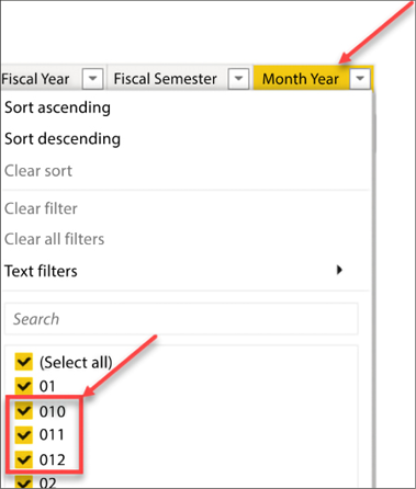
Figure 5.5: Displaying Month Year

To improve upon this and only return the two-digit month, you can use the RIGHT function. The RIGHT function returns a specified number of characters from the right side of a string; in the example below, two characters are returned from the expression. Modify your existing DAX formula to look like the following:

Month Year = RIGHT("0" & 'Date (Order)'[Month Number of Year], 2)

The rest of this formula can be completed quite easily. First, to add a dash, the following DAX code can be used:

Month Year = RIGHT("0" & 'Date (Order)'[Month Number of Year], 2) & "-"

Complete the Month Year formula by combining the current string with the Year column. The completed example is seen in Figure 5.6:

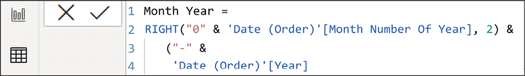
Figure 5.6: Displaying Month Year

In Figure 5.7, you see the results of the completed expression in the Date table:

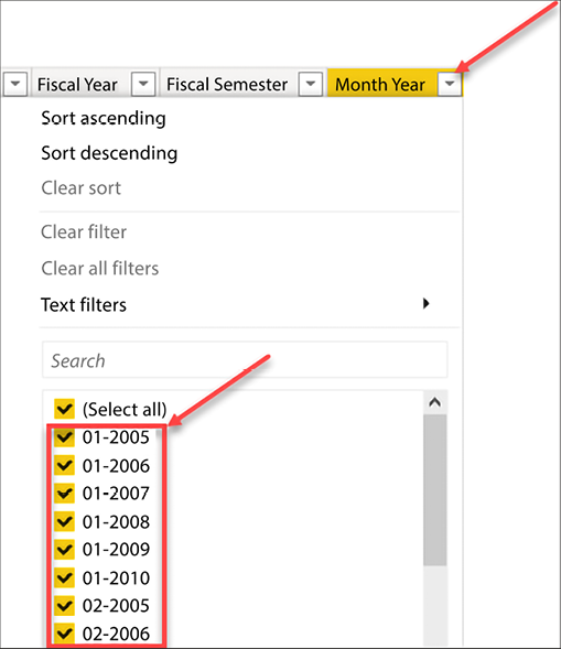
Figure 5.7: Results of the Month Year calculated column in the Date table

In this example, you learned how to create a Month Year column using a combination of the Right function with the ampersand operator. Next, you will learn an easier method for achieving the same goal with the FORMAT function.

Using the FORMAT function in DAX

As with any other language, you will find that there are usually multiple ways to do something. Now you are going to learn how to perform the calculation that we saw in the previous section using the FORMAT function. The FORMAT function allows you to take a number or Date column and customize it in a number of ways. A side effect of the FORMAT function is that the resulting data type will be text. Therefore, this may affect numerical-based calculations that you wish to perform on those columns at a later time. Let’s perform the preceding calculation again, but this time, using the FORMAT function.

Make sure you have the Date (Order) table selected, and then click on Create a New Calculated Column by selecting New column from the Table tools ribbon. In the formula bar, write the following expression:

Month Year Format = FORMAT('Date (Order)'[Date], "MM-YYYY")

Figure 5.8: Results of the Month Year calculated column in the Date table

Now, let’s take a look at the DATEDIFF function and how to implement conditional logic with the IF function in DAX.

Implementing conditional logic with IF()

Next, you are going to determine each customer’s age. The Customer table currently contains a column with the birth date of each customer. This column, along with the TODAY function and some DAX, will allow you to determine each customer’s age. Your first attempt at this calculation may be to use the DATEDIFF function in a calculation that looks something like the following:

Customer Age = DATEDIFF('Customer'[Birth Date], TODAY(), YEAR)

The TODAY function returns the current date and time. The DATEDIFF function returns the count of the specified interval between two dates; however, it does not look at the day and month and therefore, does not always return the correct age for each customer.

Let’s rewrite the previous DAX formula in a different way. In this example, you are going to learn how to use conditional logic and the FORMAT function to return the proper customer age. Please keep in mind that there are many ways to perform this calculation.

Select the Customer Age column from the previous step and rewrite the formula to look like Figure 5.9:

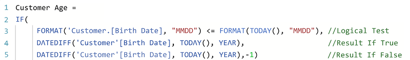
Figure 5.9: Customer Age calculation column

When completed, the preceding code returns the correct age for each customer. The FORMAT function is used to return the two-digit month and two-digit day for each date (the birth date and TODAY's date). Following the logical test portion of the IF statement are two expressions. The first expression is triggered if the logical test evaluates to true, and the second expression is triggered if the result of the test is false. Therefore, if the customer’s month and day combo is less than or equal to today’s month and day, then their birthday has already occurred this year, and the logical test will evaluate to true, which will trigger the first expression. If the customer’s birthday has not yet occurred this year, then the second expression will execute.

In this example, you learned how to implement conditional logic with the IF function. Now let’s look at the SWITCH function, which can be used as an alternative method to IF.

Implementing conditional logic with SWITCH()

Now that you have the customer’s age, it’s time to put each customer into an age bucket. For this example, there will be four separate age buckets:

• 18-34
• 35-44
• 45-54
• 55+

The SWITCH function is preferable to the IF function when performing multiple logical tests in a single DAX formula. This is because the SWITCH function is easier to read and makes debugging code much easier.

With the Customer table selected, click on New Column from the Modeling ribbon. Type in the completed DAX formula as seen in Figure 5.10:

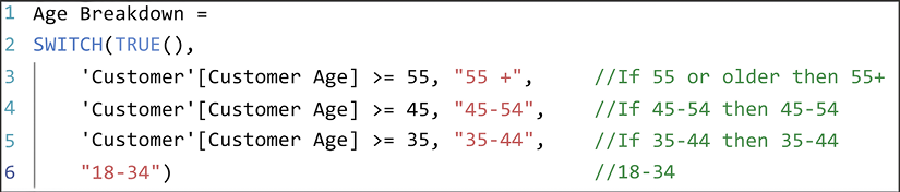
Figure 5.10: Conditional logic with SWITCH

The preceding formula is very readable and understandable. There are three logical tests, and if a customer’s age does not evaluate to true on any of those logical tests, then that customer is automatically put into the 18-34 age bucket.

The astute reader may have noticed that the second and third logical tests do not have an upper range assigned. For example, the second test simply checks whether the customer’s age is 45 or greater. Naturally, you may assume that a customer whose age is 75 would be incorrectly assigned to the 45-54 age bucket. However, once a row evaluates to true, it is no longer available for subsequent logical tests. Someone who is 75 would have been evaluated to true on the first logical test (55+) and would no longer be available for any further tests.

Let’s take a look at another important task in DAX: retrieving data from a column in another table. In Excel, you would just use the VLOOKUP function, and in SQL, you would use a join. In DAX, you use navigation functions to retrieve this data.

Leveraging existing relationships with navigation functions

It’s finally time to create a relationship between the Temperature table and the Internet Sales table. The key on the Temperature table is a combination of the region name and the month number of the year.

This column combination makes a single row unique in this table, as shown in Figure 5.11:

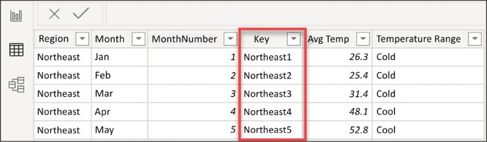
Figure 5.11: Column combination that makes a single row unique

Unfortunately, neither of those two columns currently exists in the Internet Sales table. However, the Internet Sales table has a relationship with the Sales Territory table, and the Sales Territory table has the region. Therefore, you can determine the region for each sale by doing a simple lookup operation. Well, it should be that simple, but it’s not quite that easy. Let’s take a look at why.

Calculated columns do not automatically use the existing relationships in the data model. In contrast to calculated columns, calculated measures automatically see and interact with all relationships in the data model. Now let’s take a look at why this is important. Calculated measures will be covered in the next section.

In the following screenshot, we have created a new column in the Internet Sales table and we are trying to return the region name from the Sales Territory table. Take a look at Figure 5.12:

Figure 5.12: Sales Territory table

Note that there is no IntelliSense and that the autocomplete functionality is unavailable as we type in Sales Territory. The reason for this is the calculated column creates a row context and by default does not use the existing relationships in the data model. There is a much more complicated explanation behind all this, but for now, it is sufficient to say that navigation functions (RELATED and RELATEDTABLE) allow calculated columns to interact with and use existing relationships.

If we rewrite the following DAX formula with the RELATED function, then you will notice that IntelliSense has returned, along with the autocomplete functionality that was previously discussed. The IntelliSense can be seen in Figure 5.13:

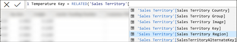
Figure 5.13: Temperature Key column

Now it’s time to create a Temperature Key column in the Internet Sales table. Create a new column in the Internet Sales table and then type in the DAX formula seen in Figure 5.14:

Figure 5.14: Temperature Key column of the Internet Sales table

You may have observed that unlike a VLOOKUP in Excel or a join in SQL, we did not have to specify the join columns when using the RELATED function! This is because the built-in navigation functions automatically leverage the existing relationships in the model.

Now that the Temperature Key column has been created in the Internet Sales table, let’s create the relationship. Click on Manage Relationships from the Home ribbon and then click on New... to open the Relationship editor window. Then, complete the following steps to create a new relationship:

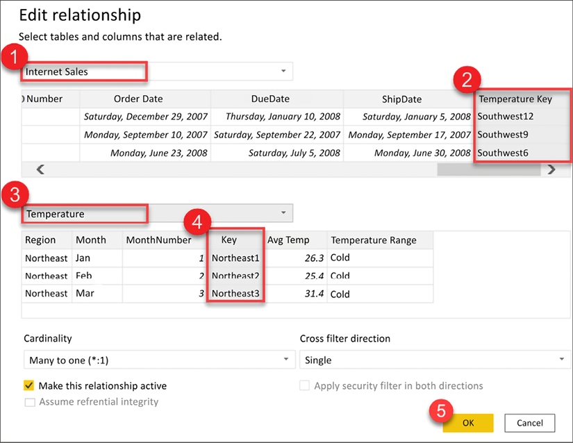
Figure 5.15: Creating a new relationship

See the numbered items in Figure 5.15:

1. Select Internet Sales from the first drop-down selection list.
2. Select Temperature Key from the list of columns (scroll right).
3. Select Temperature from the second drop-down selection list.
4. Select Key from the list of columns.
5. Click OK to save your new relationship.

So far in this chapter, you have learned how to create calculated columns in tables. These calculated columns increase the analytical capabilities of your data models by adding columns that can be leveraged to describe your metrics. You also learned how to create a concatenated key column in order to build a relationship between the Temperature and Internet Sales tables. In the next section, you are going to learn how to use DAX to create calculated measures.

Creating calculated measures

Calculated measures are very different than calculated columns. Calculated measures are not static, and operate within the current filter context of a report; therefore, calculated measures are dynamic and ever-changing as the filter context changes. You were introduced to filter context in the previous chapter when discussing many-to-many relationships. The concept of the filter context will be slightly expanded on later in this chapter. Calculated measures are powerful analytical tools, and because of the automatic way that measures work with filter context, they are surprisingly simple to author.

Before you start learning about creating measures, let’s first discuss the difference between implicit and explicit measures.

Implicit aggregations occur automatically on columns with numeric data types. You saw this in the previous chapter when the month number column was incorrectly aggregated after being added to a report. There are some advantages to this default behavior—for example, if you simply drag the Sales Amount column into a report, the value will be automatically aggregated and you won’t have to spend time creating a measure. As discussed in the next section, it is generally considered a best practice to create explicit measures in lieu of implicit measures.

An explicit measure allows a user to create a calculated measure, and there are several benefits to using explicit measures:

• Measures can be built from other measures
• Reusing measures makes the code easier to read
• They encapsulate code, making logic changes less time-consuming
• They centrally define number formatting, creating consistency

Calculated measures can do the following:

• They can be assigned to any table and further assigned to folders within that table
• They interact with all the relationships in the data model automatically, unlike calculated columns
• They are not materialized in a column, and therefore cannot be validated in the Data View

Now that you know what calculated measures are, let’s take a look at how to create them.

Creating basic calculated measures

In this section, you are going to create four simple calculated measures. These calculated measures will create additional metrics that can be used in visualizations and reports to obtain deeper insights from your data:

• Total Sales
• Total Cost
• Profit
• Profit Margin

First, let’s start by creating the Total Sales calculation.

Total Sales

To create your first measure, select the Internet Sales table and then click on New measure from the Table tools ribbon. Insert the following code in the formula bar:

Total Sales = SUM('Internet Sales'[Sales Amount])

See Figure 5.16:

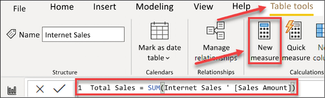
Figure 5.16: Create a Total Sales measure

One of the benefits of creating explicit measures is the ability to centralize formatting. Once the measure has been created, navigate to the Measure tools ribbon and change the formatting to $ English (United States), as shown in Figure 5.17:

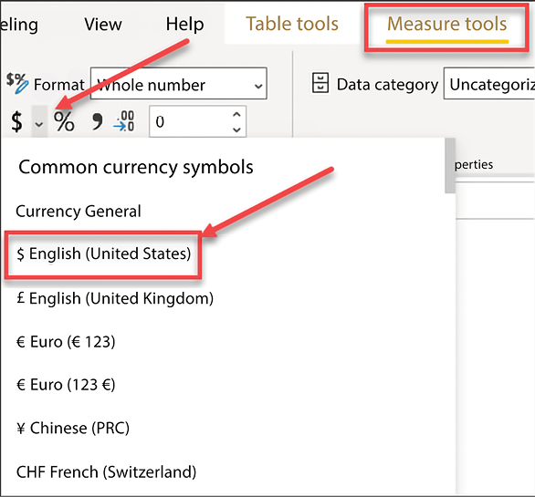
Figure 5.17: Change formatting to $ English (United States)

You just created your first calculated measure! It was simple and, as you will soon learn, extremely powerful. The total sales calculation is the sum of the sales amount, however, another way to read that calculation is the sum of the sales amount within the current filter context. You learned about filter context in the previous chapter and it will be further discussed later in this chapter, but for now, just know these seemingly simple calculations are very dynamic. Let’s create some more calculated measures.

Total Cost

Now let’s create the Total Cost measure. Once again, this is a simple SUM operation. Select the Internet Sales table, then click on New measure from the Table tools ribbon and type in the following DAX formula:

Total Cost = SUM('Internet Sales'[Total Product Cost])

Remember to apply formatting to this new measure; it is easy to miss this step when learning to create measures. The formatting should be $ English (United States).

Profit

Profit is the next measure you will create. You may attempt to write something such as the following:

Profit = SUM('Internet Sales'[Sales Amount]) - SUM('Internet Sales'[Total Product Cost])

This calculation would be technically correct; however, it is not the most efficient way to write code. In fact, another benefit of building explicit measures is that they can be built using measures you already created. Reusing existing calculated measures will make the code more readable and make code changes easier and less time-consuming. Imagine for a moment that you discovered that the Total Sales calculation is not correct. If you encapsulated all this logic in a single measure and reused that measure in your other measures, then you need only change the original measure, and any updates will be pushed to all other measure references.

Now it is time to create the Profit measure. Select your Internet Sales table and then click on New measure from the Table tools ribbon. Type the following into the formula bar—remember to apply formatting afterward:

Profit = [Total Sales] - [Total Cost]

This calculation returns the same results as the original attempt. The difference is that now you are reusing measures that were already created in the data model. You may have noticed that I referenced the name of the measure without the table name. When referencing explicit measures in your code, it is considered a best practice to exclude the table name.

Profit Margin

Now it’s time to create the Profit Margin calculation (the profit margin is simply (profit/sales). For this measure, you are going to use the DIVIDE function. The DIVIDE function is recommended over the divide operator (/) because the DIVIDE function automatically handles divide-by-zero occurrences. In the case of divide-by-zero occurrences, the DIVIDE function returns blank.

Create a new measure in the Internet Sales table using the following code:

Profit Margin = DIVIDE([Profit], [Total Sales])

Next, set the formatting as a percentage. From the Modeling ribbon, click on the % icon, as shown in Figure 5.18:

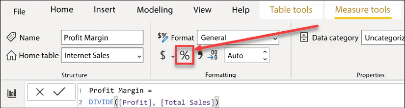
Figure 5.18: Setting formatting as a percentage

Functions in DAX have required and optional parameters. So far, you have only learned about required parameters. Let’s take a look at optional parameters.

Optional parameters

You may have noticed that the DIVIDE function accepted three parameters and you only provided two. The third parameter allows you to set an alternative result for divide-by-zero occurrences. This alternate result is optional. Optional parameters are denoted by square brackets on both sides of the parameter. These optional parameters are prevalent in many DAX functions. Take a look at Figure 5.19:

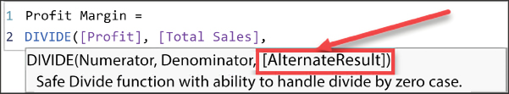
Figure 5.19: Optional parameters in DAX functions

Optional parameters are very often overlooked by developers, but as you will learn, there is a lot of functionality and value that can be achieved by leveraging these parameters. Now, let’s take a look at how and where to assign calculated measures.

Assignment of calculated measures

Unlike calculated columns, measures do not need to be assigned to a specific table to function properly. Because of this, it is very easy and common to forget to make sure the proper table is selected prior to creating a measure. This results in measures being assigned to random tables during development.

Fortunately, you do not need to delete the measure and recreate it in the proper table; instead, you can simply move measures from one table to another by changing the Home table.

To move a calculated measure from one table to another, you will follow these steps, as you can see in Figure 5.20:

1. Select the measures.
2. Find the Measure tools ribbon.
3. Click on the Home table dropdown and select the correct table:

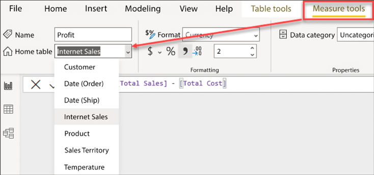
Figure 5.20: Moving a calculated measure to a new table

Calculated measures can be assigned to any table in your data model and will still function properly. However, measures should be assigned to the table where it logically makes the most sense. This way, the measure is easy to find and utilize in visualizations and reports. Let’s take a look at how measures can be logically organized and grouped into folders.

Display folders

In Power BI, columns and measures can be assigned to folders. This is extremely useful for organizing related measures and improving the overall usability of the data model. By properly leveraging display folders, measures will be easier to find and similar measures, like time intelligence calculations, can be grouped in their own folder.

As you can see in Figure 5.21, the newly created measures are mixed in with the existing columns:

Figure 5.21: Calculated measures displayed in a table

At the time of writing, adding measures to display folders can only be accomplished from the Model View. Select Model View from the left navigation pane. Next, expand the Internet Sales table and select the Profit measure. Finally, in the Properties pane, find the Display folder property and type Measures. Take a look at Figure 5.22:

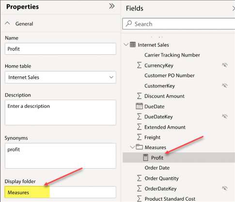
Figure 5.22: Calculated measures displayed in a table

All of your measures can be moved to a display folder at one time. Simply multi-select the measures to be moved by holding down the Ctrl key while selecting each measure and then enter the folder name. See the completed example in Figure 5.23:

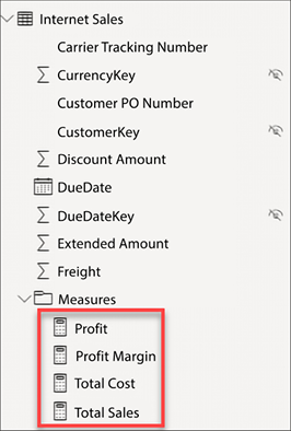
Figure 5.23: Displaying measures in a folder

Previously, we mentioned that these calculated measures are simple yet powerful. These measures are powerful because filtering in DAX occurs automatically. Let’s take a deeper look at automatic filtering and filter context.

Understanding filter context

The automatic filtering that occurs in Power BI is a really awesome feature and is one of the reasons that so many companies are gravitating to this tool. The active relationships that are defined in the data model, and that you learned how to create in the previous chapter, are automatically used by DAX to perform the automatic filtering of calculated measures. This is directly tied to the concept of the filter context. You were introduced to the filter context in the previous chapter. I want to briefly expand on what was covered in the previous chapter here before discussing the CALCULATE function.

A simple definition of the filter context would be that it is simply anything in your report that is filtering a measure. There are quite a few items that make up the filter context. Let’s take a look at a few of them:

• Any attributes on the rows; this includes the different axes in charts
• Any attributes on the columns
• Any filters applied by slicers (visual filters); slicers are discussed in the next chapter
• Any filters applied explicitly through the Filters pane
• Any filters explicitly added to a calculated measure

In short, the filter context makes the authoring of calculated measures a simple and intuitive process. A simple total sales calculation can be automatically filtered by all the tables in your data model without having to write any additional logic into your calculated measures. If you want to see total sales by customer, product name, product weight, country, or any other number of columns in your data model, simply add that column to your report and your measure is auto-magically filtered thanks to the active relationships!

Using CALCULATE() to modify filter context

The CALCULATE function is an extremely powerful tool in the arsenal of any DAX author. In fact, the CALCULATE function is one of the most important functions in all of DAX. This is because the CALCULATE function can be used to ignore, overwrite, or change the existing filter context. You may be asking yourself why—why would anyone want to ignore the default behavior of Power BI? Let’s take a look at an example.

Let’s assume you want to return the total sales of each country as a percentage of all countries. This is a very basic percentage of total calculation: Total Sales per country divided by Total Sales for all countries. However, how do you get the total sales of all the countries so that you can perform this calculation? This is where the CALCULATE function comes into the picture. Take a look at Figure 5.24:

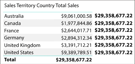
Figure 5.24: Calculating the total sales of all the countries

To do the percentage of total calculation, you first need Total Sales all Countries on the same row as Total Sales. Therefore, you need to create a new calculated measure that ignores any filters that come from the Country attribute. Create a new calculated measure in your Internet Sales table using the following DAX formula:

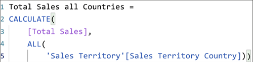
Figure 5.25: Use CALCULATE to ignore filters from Country

The calculation in Figure 5.25 will return all sales for all countries, explicitly ignoring any filters that come from the Country column. Let’s briefly discuss how and why this works.

The first parameter of the CALCULATE function is an expression, and you can think of this as an aggregation of some kind. In this example, the aggregation is simply Total Sales. The second parameter is a filter that allows the current filter context to be modified in some way. In the preceding example, the filter context is modified by ignoring any filters that come from the Country attribute. Let’s take a look at the definition for the ALL function used in the second parameter of the CALCULATE function:

ALL: Returns all the rows in a table, or all the values in a column, ignoring any filters that may have been applied.

Alternatively, the REMOVEFILTERS function can be used instead of ALL to achieve the same results. For this example, these functions can be used interchangeably. I find that most developers new to DAX find REMOVEFILTERS a bit easier to understand. Modify the measure created in the last step, Total Sales all Countries, to use REMOVEFILTERS instead of the ALL function, as you can see in Figure 5.26:

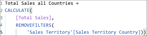
Figure 5.26: Replace the ALL function with REMOVEFILTERS

The most difficult challenge to creating our percentage of total calculation in DAX is creating the total sales for all countries. With this calculated measure completed, let’s complete the percentage of the total calculation.

Calculating the percentage of total

Now, create another calculated measure in the Internet Sales table using the following code. Make sure that you format the measure as a percentage:

% of All Countries = DIVIDE([Total Sales], [Total Sales all Countries])

In Figure 5.27, you can see the completed example with both of the new measures created in this section. Without a basic understanding of the CALCULATE function, this type of percentage of total calculation would be nearly impossible:

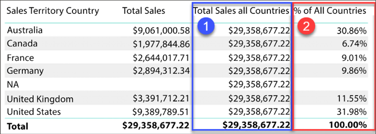
Figure 5.27: Completed example with new measures

In Figure 5.27, you may notice that a new row with the value of NA appeared in the column Sales Territory Country. Previously, this NA value was automatically hidden by the Power BI visual because Total Sales returned a blank value. However, Total Sales all Countries will ignore the NA filter and return total sales for all countries and therefore, the NA value now appears in the table visual.

In this section, you were introduced to the CALCULATE function in DAX. The default filters that are applied in Power BI are awesome, but sometimes you need the ability to evaluate an expression, like total sales, in a modified filter context, and the CALCULATE function is perfect for that.

Working with time intelligence functions

Another advantage of Power BI is how easily time intelligence can be added to your data model. DAX has a comprehensive list of built-in time intelligence functions that can be easily leveraged and add significant analytical value to your data model. In this section, you are going to learn how to use these built-in functions to create the following measures:

• Year to Date Sales
• Year to Date Sales (Fiscal Calendar)
• Prior Year Sales

In order to leverage time intelligence functions in DAX, you must have a date table in your data model and that date table must have all available dates with no gaps. These are very important conditions that must be met. Oftentimes, developers try to use the date column from their transaction table (fact table). This can result in calculations that do not work and return incorrect results. In the previous chapter, you learned how to properly build a relationship from your date table to your fact table and multiple methods for marking your date table as a date table. Now that we have added some clarity here, let’s create a year-to-date sales calculation.

Creating year-to-date calculations

Create a new calculated measure in your Internet Sales table using the following DAX formula. See the results in Figure 5.28 below. Remember to format the measure as $ English (United States):

YTD Sales = TOTALYTD([Total Sales], 'Date (Order)'[Date])

Maybe your requirement is slightly more complex, and you need to see the year-to-date sales based on your fiscal year end rather than the calendar year-end date. The TOTALYTD function has an optional parameter that allows you to change the default year-end date from 12/31 to a different date. Create a new calculated measure in your Internet Sales table using the following DAX formula:

Fiscal YTD Sales = TOTALYTD([Total Sales], 'Date (Order)'[Date], "03/31")

Now, let’s take a look at both of these new measures in a table in Power BI:

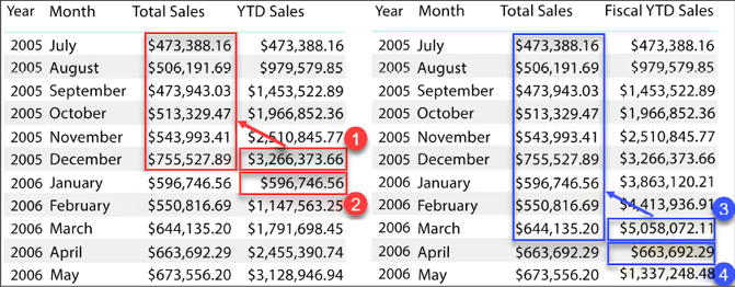
Figure 5.28: Comparing YTD Sales with Fiscal YTD Sales

The newly created measures YTD Sales and Fiscal YTD Sales have both been added to the preceding table. Let’s take a closer look at how these two measures are different; the relevant sections in the table are annotated with the numbers one to four, corresponding to the following notes:

1. The amount displayed for December 2005 is $3,266,374.66 This is the cumulative total of all sales from January 1, 2005 to December 31, 2005.
2. As expected, the cumulative total starts over as the year switches from 2005 to 2006; therefore, the YTD Sales amount for January 2006 is $596,747.
3. In the Fiscal YTD Sales column, the cumulative total works slightly differently. The displayed amount of $5,058,072.11 is the cumulative total of all sales from April 1, 2005 to March 31, 2006.
4. Unlike the YTD Sales measure, the Fiscal YTD Sales measure does not start over until April 1. The amount displayed for April 2006 of $663,692.29 is the cumulative total for April. This number will grow each month until May 31, at which point, the number will reset again.

In this section, you learned about a built-in time intelligence function in DAX; there are many of these functions that make doing time series analysis much easier. Now let’s take a look calculating a prior year sales calculation.

Creating prior year calculations with CALCULATE()

A lot of time series analysis consists of comparing current metrics to the previous month or the previous year. There are many functions in DAX that work in conjunction with the CALCULATE function to make these types of calculations possible. In this section, you are going to create a new measure to return the total sales for the prior year.

Using Figure 5.29 as a reference, create a new calculated measure in your Internet Sales table for Prior Year Sales:

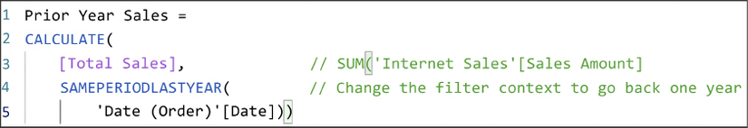
Figure 5.29: Create a Prior Year Sales calculation

CALCULATE allows you to ignore or even change the current filter context. In the preceding formula, CALCULATE is used to take the current filter context and modify it to one year prior. This calculated measure also works at the day, month, quarter, and year levels of the hierarchy. For example, if you were looking at sales for June 15, 2020, then the Prior Year Sales measure would return sales for June 15, 2019. However, if you were simply analyzing your sales aggregated at the month level for June 2020, then the measure would return the sales for June 2019.

In this section, you learned how to add time series analysis to your data model, adding significant analytical value and allowing you to extract valuable insights from your data across time. In other programming languages, it would take significant amounts of code and an in-depth validation process to perform the same calculations that can be achieved in DAX with minimal effort.

Role-playing tables with DAX

In Chapter 4, Building the Data Model, you learned how to develop your data model to deal with role-playing tables, by importing a table multiple times. We mentioned then that there was an alternative method using DAX. In this section, we will explore this alternative method and the pros and cons of using DAX versus the method you have previously learned.

Since leveraging DAX does not require importing a table multiple times, you will immediately gain savings on storage and, unlike the other method, with DAX, you will not need to manage multiple tables in Power BI Desktop.

The DAX method requires that inactive relationships be created in order to work correctly. Inactive relationships are not often used in DAX because they are not used automatically like active relationships. Unlike active relationships, you can have more than one inactive relationship between two tables.

Let’s create a new relationship between the Internet Sales table and the Date (Order) table. First, open the relationship editor by referring to Figure 5.30 and the steps following:

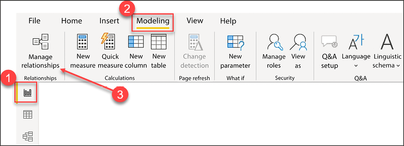
Figure 5.30: Launch the Manage relationships dialog box

1. Navigate to the Report View.
2. Select the Modeling ribbon across the top of Power BI Desktop.
3. Click on Manage relationships.

Once the Manage relationships box appears, click on New… to create a new relationship. Continue creating the relationship with the steps by referring to Figure 5.31 and the steps following:

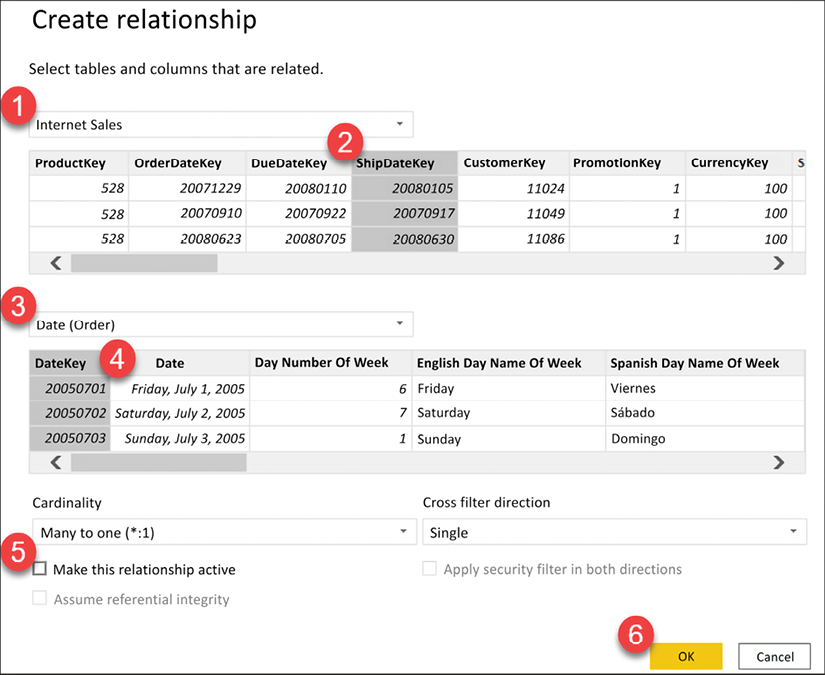
Figure 5.31: Create the inactive relationship between Internet Sales and Date (Order)

1. Select Internet Sales from the drop-down menu.
2. Select the ShipDateKey column from the list of columns.
3. Select Date (Order) from the drop-down menu.
4. Select the DateKey column from the list of columns.
5. Do not select Make this relationship active.
6. Click OK.

The new relationship can be observed in Figure 5.32, which is a screenshot of the Manage relationships dialog box:

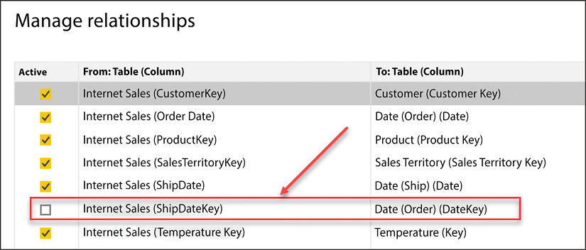
Figure 5.32: New relationship between Internet Sales and Date (Order)

Now that the inactive relationship has been created, we can create the calculated measure to return Total Sales by Ship Date. The completed calculated measure can be seen in Figure 5.33:

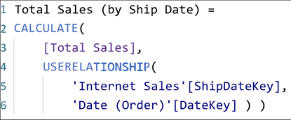
Figure 5.33: New calculated measure

This measure will make use of two functions in DAX. First, the CALCULATE function is used here because the filter context is going to be modified to use the inactive relationship rather than the active relationship. Second, the USERELATIONSHIP function specifies that the Internet Sales table should be filtered by ShipDateKey rather than the active relationship on OrderDateKey.

The completed measure can be seen in Figure 5.34 along with the original Total Sales calculation:

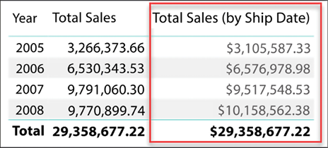
Figure 5.34: Validating the new calculated measure

In Figure 5.34, the Total Sales measure is returning the total sales based on the active relationship in the data model, which is on OrderDateKey, therefore $3,266,373 is returned for the year 2005. Alternatively, the Total Sales (by Ship Date) measure is returning $3,105,587.33 in sales.

This approach does not require importing additional tables and therefore is superior to the method you learned in Chapter 4, Building the Data Model, for optimizing space in your data model. However, with the DAX method, you would be required to create a new measure for every measure in your data model that you wanted to see by the Ship Date. Therefore, if you had 50 measures in your table, you would create a new version of each of those measures and would specify that the new measure should use the inactive relationship on ShipDateKey rather than the current active relationship. Because of this reason alone, the method you learned in Chapter 4, Building the Data Model, is the most common approach to handling role-playing tables.

In this section, you learned an alternative method to provide support for role-playing tables in Power BI Desktop. This method has historically required significantly more development effort and therefore has not been as popular as the method you learned previously.

As we bring this chapter to a close, I feel it’s necessary to mention that there are several developer-friendly tools that can help the DAX developer gain better insights into their data models. These tools are outside the scope of this book, but as you continue your journey with DAX, you will want to learn more about DAX Studio and the Tabular Editor.

Summary

In this chapter, you learned that DAX allows you to significantly enhance your data model by improving the analytical capabilities with a relatively small amount of code. You also learned how to create calculated columns and measures and how to use DAX to perform useful time series analysis on your data.

This chapter merely scratched the surface of what is possible with DAX. As you further explore the DAX language on your own, you will quickly become a proficient author of DAX formulas. As with everyone who learns DAX, you will inevitably learn that there is a layer of complexity to DAX that will require further education to really master. When you get to this point, it would be advantageous to look for classes or books that will help you to take your skills to the next level and truly master DAX!

Join our community on Discord

Join our community’s Discord space for discussions with the authors and other readers:

https://packt.link/ips2H