6

Determining Requirements and Specification Models

6.1. Introduction

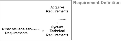
As pointed out in the previous chapter, the composition of a technological system is made up of building blocks that its endo-structure assembles, as shown in Figure 5.2. For each building block, the same design process is applied, except for the terminal blocks, to which a specific process is applied.

The design process of each block consists of two subprocesses:

The first of subprocess involves the following tasks:

Figure 6.1. EIA632 building block requirement definition subprocess

The second subprocess, called the design solution process, will be dealt with in the next chapter, whereas the current chapter is dedicated to the determination of requirements, that is to say, establishing the specification of requirements assigned to a system.

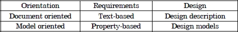
In the property-model methodology approach, which is based on models, such requirement specifications are called specification models. We will associate with the considered type of systems, and its subsystems, specification models, as already recommended in the EIA 632 standard.

Instead of specification documents written using tools such as Microsoft Word, IBM DOORS and others, the specificity of property-model methodology (PMM) lies in specification models that are compiled and executable in simulation environments, when they are subjected to simulation scenarios.

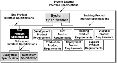
Figure 6.2. EIA632 system specification architecture

We will introduce here the concepts of systems specification, overspecification, underspecification and exact specification. After considerations of the subjective character of text-based requirements (TBRs) and text-based specification, we will introduce the concept of property-based requirement (PBR). On this concept, we will develop a theory of these PBRs, which is consistent with the model-based systems engineering (MBSE) paradigm. In particular, we will define a partial-order relation (comparison of requirements) and a conjunction operator among requirements, based on Bunge’s theory of properties¹ (see section 1.5.2). We will then present an interpretation process that allows us to translate TBR into one or more PBRs. We will give examples of this interpretation process of TBRs coming from the regulations. We will conclude this chapter with a discussion on the relationship between specification models and concurrent assertions of simulation languages.

In Chapter 7 (section 7.2), we will introduce the concept of requirement derivation, whereas in later chapters, we will deduce, from them, two theorems of practical importance: the first (mentioned in section 9.3.5) which we call the contract theorem assures the conformity of a system, under certain conditions, with its specification model, whereas the second theorem (mentioned in section 10.3.7) concerns the impact of additional requirements introduced at a subsystem level, on the feasibility and safety of a type of systems.

6.2. Specifications and requirements

Here, we consider a collection of concrete objects composing a reference collection² K, for example, the collection of geostationary artificial satellites or the collection of transport helicopters or even the collection of nuclear power plant units.

Specifying a collection E of entities of type K, to be developed, means defining well-formed requirements {Req_i}_1≤i≤n, such that any entity e belongs to E if and only if e simultaneously satisfies all the requirements Req_i of {’}_1≤i≤n.

This can be formalized as follows: E=SAT_K({Req_i}_1≤i≤n) where SAT_K({Req_i}_1≤i≤n denotes the collection of entities of type K that shall satisfy the requirement specification {Req_i} _1≤i≤n

Now let us consider a collection E of entities of type K and a specification S ={Req_i}_1≤i≤n:

It is incredibly easy to produce inaccurate specifications; practice shows us this repeatedly. This is why a specification shall be validated, as already mentioned with standards such as EIA 632 or an aeronautical recommendation such as ARP4754A. The validation process discussed in Chapter 8 is a process that aims to produce specifications as exact as possible.

Clearly, there may be many ways to specify a collection E of entities to be developed. We then obtain: E = SAT_K({Req_i}_1≤i≤n)=SAT_K({Req_j}_1≤j≤m), and the specifications {Req_j}_1≤j≤n and ({Req_i}_1≤i≤m) are then technically equivalent. However, these technically equivalent specifications may not be equivalent from an economic point of view. Some of them may be less costly to develop than others.

Intuitively, we can think that even if they are technically equivalent, the specifications with a limited number of requirements, which are comprehensible and easy to implement and test, are more desirable than specifications with many requirements, which are difficult to understand, implement and test. The second type of specifications are more complicated and costly than that of the first type.

The purpose of determining the requirements of a collection E of entities is to define an exact specification S of E that is as simple as possible. This is our objective in this chapter.

6.3. Text-based requirements and subjectivity

Usually, a requirement is defined as a statement that expresses either an obligation or a prohibition. One of the most consistent definitions is provided by the IEEE 1220 standard [IEE 05] which specifies that a requirement is “a statement that identifies a product or process operational, functional, or design characteristic or constraint, which is unambiguous, testable or measurable, and necessary for product or process acceptability (by consumers or internal quality assurance guidelines)”. Other standards (e.g. EIA 632, ISO15288 and ARP4754A) are much more vague with regard to the definition of “requirement”. In particular, ISO15288 does not define the term and ARP4754A is a good example of a window dressing (trompe l’oeil) definition: to show this point, it is sufficient to compare the definition of a requirement (“requirement: an identifiable element of a function specification that (..)” to that of a specification (“specification: a collection of requirements which (..)”).

Moreover, there is a great amount of publications on the art of writing good requirements, revealing the difficulty to produce requirements of good quality. In 1796, Joseph de Maistre had already highlighted in his Considérations sur la France that “it is much less difficult to solve a problem, than to define it”. This difficulty seems to increase when a natural language is used as a specification means. Natural languages due to their polysemic richness leave the door wide open to all ambiguities, misinterpretations and all that is implied and unspoken. This is what each engineer may experience daily, especially when he/she works in a context spread over several geographic, linguistic and cultural areas.

The question that this observation asks is the following: is the statement of requirements in a natural language (more or less coded), which we call TBR, efficient and for which cost? Basically, are TBRs not too subjective productions to allow a shared understanding between all stakeholders of the problem to be solved? Would it not be better constrain the expression of a requirement until it is completely unambiguous, in other words, until it can be processed by a computer?

We claim that the most efficient way of obtaining requirements, which as IEEE 1220 indicates are unambiguous, testable or measurable, at a reasonable cost, is to give an objective expression of them that does not leave any room for interpretation in the signification of this expression. Moreover, we assert that this objectivity is necessary for an MBSE approach. The MBSE approach of systems engineering poorly accommodates TBR engineering. The reason for this discordance is due to the fact that TBR engineering is consistent with a systems engineering approach that focuses on documents, it shares the same engineering vision, of the same scientific paradigm (using a buzzword that made the fame of Kuhn [KUH 70]).

What we propose here is a formalized approach of requirements, which we called PBRs to emphasize the relationship with the concept of property, widely mentioned in the “foundations” part of this book (see section 1.5).

We consider that this requirement engineering approach is based on the same paradigm as that of the MBSE approach. This is why we define the set of PBRs assigned to an entity such as the specification model of this entity.

Table 6.1. Document-centric versus model-centric paradigms

6.4. Objectifying requirements and assumptions through property-based requirements

We claim that the theory of PBRs is a feasible and economic method for solving problems caused by the subjectivity of text-based specifications and a means for reducing the disorder entailed by this subjectivity in system development processes. The theory of PBRs is a theory of objective specifications.

6.4.1. Definition

We call PBR, concerning a type of systems Σ, a constraint enforced on some property P of Σ. This constraint enforces that the values of property P are in a domain D when condition C is fulfilled, provided that Im(P) is the domain of possible values of P and D is a strict subset of Im(P). This definition can be formalized as follows:

PBR: [when C] → val(O.P) ∈ D⊂Im(P)

In this expression, the term PBR is a label that identifies the requirement; this label is mandatory.

In the optional expression [when C] (signaled by the presence of brackets []), the term C denotes the condition of actualization (Boolean expression that may be true or false) that is relevant in the context in which the requirement is expressed. Condition C may denote, for example, a state, an event and a mode (see these terms in section 2.5) of a system belonging to the type of systems Σ, or a state or even an event of its environment.

The term O denotes a concrete object or a type of concrete objects. Object O may be Σ itself or one or several elements of its composition C, environment E or structure S. P is a material property of this object or this type of objects. The domain of possible values of this property is called the image of P and is denoted by Im(P), and thus the domain of values D indicated by the requirement is such that D is strictly included in Im(P) (i.e. D ⊂ Im(P)). Therefore, the expression, which reads as the values of property P of object O (val(O.P)), shall be in domain D, which is a strict subset of the image of P.

Im(P) is a set determined by the definition of property P. If P is a qualitative property, then Im(P) is a finite set {a₁, ..,a_n}; otherwise if P is a quantitative property, then Im(P) may be a countable or an unaccountable part of , where n is a positive integer.

In summary, the PBR requirement above means that “when condition C is met, the values of property P of object O shall be in the subset D of Im(P)”.

Note that the PBR requirement does not say anything about what is to happen when condition C is not satisfied.

Therefore, when condition C is met and the value of O.P is not in domain D (i.e. val(O.P) ∈ Im(P)-D), we say that the PBR requirement is not satisfied or is breached.

Also note that the requirement:

PBR: [when C] → val(O.P) ∉ D⊂Im(P)

is identical to the requirement:

PBR’: [when C] → val(O.P) ∈ Im(P)-D

In other words, a PBR allows both an obligation and a prohibition to be expressed in the same way.

Moreover, we say that a PBR is an assumption regarding the type of systems Σ denoted by (C,E and S), if O is an object belonging to environment E of this type of systems Σ. This distinction, which was introduced in the initial versions of KAOS [LET 02], and unfortunately, subsequently abandoned, helps differentiate between constraints assigned to the composition and the structure of the system on which designers may act and those assigned to the environment to which the designer is subjected.

6.4.2. Examples

Note that SAT_K({PBR_i}_i∈I) refers to a collection of type K systems that satisfy the set of PBR_i when i belongs to I. For example, we can consider the collection of transport HC helicopters with at least 10 passenger seats, autonomy of at least 200 miles and a direct operating cost less than $1,500, which allows us to define three PBRs:

PBR₁: val(HC.Passenger_seat_number) ≥ 10;

PBR₂: val(HC.range) ≥ 200 nm;

PBR₃: val(HC.Direct_Operating_Cost) ≤ $1,500.

We are then able to complete this first specification without any particular problem by adding some PBRs. The only questions that remain to be answered are, on the one hand, whether they are necessary (and from which point of view?) and, on the other hand, will a multiplication of PBRs not cause infeasibility (this concept is already defined in section 6.2).

For example, we can add a maximum rate of climb requirement such as:

PBR₄: val(HC.MaxVz) ≥ 1,750 ft/min

or a maximum velocity such as:

PBR₅: val(HC.MaxSpeed) ≥ 180 mph

Furthermore, when designing a type of systems, we may need to determine important characteristics including, for example, a never exceed speed (VNE) and the takeoff decision point (TDP). Determining these characteristics is imposed by the regulations. However, these requirements are not assigned to the type of systems itself but to the development and certification processes for the type of systems. In other words, these requirements are assigned to the Design Office, which is the designing system³ for the type of systems considered.

Similarly, other regulatory requirements may constrain the operation of a type of systems, such as the operation rule requiring to never exceed the velocity never exceed (VNE), or the one requiring to reject a takeoff, in the event of one engine failure occurring before the take-off decision point (TDP), and to continue beyond this point to complete the whole takeoff path. These are, therefore, requirements assigned to the operating process for the type of systems considered and are included in pilot’s handbooks or flight manuals (here, the enabling system is the pilot).

However, these requirements, assigned to the operation process of the type of systems considered, may in turn be reassigned to systems supporting operations, such as an autopilot, which will never permit the VNE to be exceeded when it is engaged and can be formalized as follows:

PBR₆: when AFCS_engaged → val(HC.AirSpeed) ≤ VNE − threshold

Similarly, continued takeoff when one engine failure occurs beyond the TDP and the emergency procedure is properly applied by the pilot presupposes that the aircraft has the capability to achieve this goal.

PBR₇:when HCtakingOff and OEIafterTDP and OEItakeOffEmergProcedure=OK
→ val(HC.TakeOff_PathPerformance) = Successful

6.4.3. Typology and sources of PBR

The previous examples provide us with the opportunity to suggest a typology of PBR that is both justified and coherent and clarify two concepts that are often confused, the type of a requirement and source of a requirement.

In fact, the guides (e.g. SEBOK v1.2, p. 228 [SEB 13]) and standards (ISO/IEC/IEEE 29148:2011, ED79A/ARP4754A) often provide classifications (also called taxonomies and typologies) that mix the two aspects (sources and types) and do not define a typology in the strict signification⁴ of the term.

For example, ISO/IEC/IEEE 29148 [ISO 11] introduces the following types of requirements (section 5.2.8.2, p. 14):

In this context, it is difficult to claim, on the one hand, that an individual requirement shall be complete (section 5.2.5, p. 11) and, on the other hand, characterizing (section 5.2.8.2, p. 14) a performance requirement as “a requirement that defines the extent or how well, and under what conditions, a function or task is to be performed”, which means that a performance requirement completes the characterization of a functional requirement (which is, therefore, not complete when it lacks performance attributes).

Similarly, quality requirements, such as the reliability of services provided by a system (for example, the probability of indicating an undetected erroneous altitude will be less than 10^-9 per flight hour), come clarify and objectify some aspects of a functional requirement, which in their absence, would remain without content (here, indicating altitude). It is, therefore, unusual to place them into a “non-functional” category as is done in ISO/IEC/IEEE 29148 p. 14.

We can provide multiple examples to show that this type of classifications is not robust, and it is not based on well-defined classification criteria, but rather on empirical inventories⁵, which in practice lead to damaging situations, where two designers classify the same requirement into different categories, such as “the following flight data (..) shall be registered for maintenance purposes” which may be classified by a designer as a maintainability requirement (and, therefore, non-functional), whereas another may classify it as a functional requirement of a flight data recording system.

Our theory of PBRs clarifies this situation.

We call the sources of a given requirement the stakeholders who express this requirement vis-à-vis of one type of systems. These sources may be the acquirer (the client - operator - or its substitutes: marketing and client support of the company) or other stakeholders (certification authority and speciality engineers - certification, safety, costs, environmental conditions, design, production, tests, maintenance and training entities, etc.). It is always useful to be able to relate a requirement to its source without forgetting that the requirement may have multiple sources and that this connection does not predetermine any type of requirement.

In addition, there are three and only three types of PBRs assigned to a system, namely:

6.4.3.1. Structural requirements

We call structural PBR, any PBR that concerns a structural property of a system (see Chapter 1), namely its composition and structure.

The examples of structural PBR include (1) a PBR concerning the presence or absence of such and such a component; (2) a PBR about the shape, composition of a component and its dimensions; (3) PBR on the presence or absence of redundancies, on the number of inputs or outputs and (4) a PBR concerning the physical quantities that characterize its state (mass, inertia, impedance, etc.).

Figure 6.3. Airfoil structural properties and related PBR

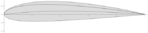
Therefore, the requirements concerning the following wing characteristics composed of structural requirements, area, thickness, camber, lift and drag coefficients, are ultimately summarized in a National Advisory Committee for Aeronautics (NACA) profile.

6.4.3.2. Behavioral requirements

We call behavioral PBR, any PBR about a behavioral property of a system, namely its behavior (most frequently elided in its observable behavior). Thus, PBRs on lift force, drag force or wing speed in an air mass are examples of behavioral PBRs.

Due to the laws of fluid mechanics, behavioral and structural properties of a wing are linked to each other by relations such as L = 1/2 ρC_LSv² where L and v are behavioral properties, whereas ρ, C_L and S are structural properties of the air mass or wing (as defined in section 1.5.3; this interdependence is characteristic of the essential properties of an object). These real links between the essential properties are a condition of possibility of engineering activities. Consequently, couplings between structural and behavioral requirements about the essential properties of an object exist. These couplings between requirements may cause unfeasibility. When this is the case, we say that the corresponding requirements are conflicting.

6.4.3.3. Mixed requirements

As we will see in the next section, it is possible to combine PBRs using a conjunction operator, in other words, to define the conjunction of two or several PBRs as a PBR. This brings us to introduce a third type of PBR namely mixed PBR. A mixed PBR is a conjunction of structural and behavioral PBRs.

An example of a mixed PBR would be an interface PBR that fixes both structural (geometric, mechanic and electrical characteristics) and behavioral characteristics communication and transmission speed protocols and error handling) of an interface.

6.5. Conjunction and comparison of property-based requirements

In this section, we are going to introduce two surprisingly new concepts of requirement engineering that are also rather “natural”. The first concept is a comparison relationship between PBRs, called “is less constraining than”, and the second concept is an operator between PBRs: the conjunction of two PBRs.

6.5.1. Comparison of two PBRs

Let us consider the following PBRs: PBR₁: val(HC.Passenger_seat_number) ≥ 10, namely a type HC of helicopters, to be developed, shall provide at least 10 passenger places. We can see that this requirement is clearly less constraining than the following requirement: PBR₂: val(HC.Passenger_seat_number) ≥ 12, i.e. “that can the most, can the least” and that an aircraft capable of transporting 12 people can, a fortiori, only transport 10 passengers.

To express that PBR₁ is less constraining than PBR₂’, we can write: PBR₁ ≤ PBR₂. Similarly, we can say that, if an object of type HC satisfies the requirement PBR₂ then, a fortiori, this object satisfies the requirement PBR₁. We can also say that SAT_K(PBR₂) ⊂ SAT_K(PBR₁). In other words, the less constraining a requirement is, the more objects there are that are capable of responding to it, i.e. logically, the intension of a predicate is the inverse of its extension.

This brings us to the following definition:

PBR₁ ≤ PBR₂ ⇔ SAT_K(PBR₂) ⊂ SAT_K(PBR₁)

What results is that the more constraining a requirement is, the more the space of solutions satisfying this requirement is reduced. This makes sense, but deserves to be formalized.

In particular, if SAT_K(PBR)=∅, then there is no object of type K that meets this PBR. In this case, we are confronted by an unfeasibility (see section 6.2.).

Similarly, we can say that requirements {PBR_i}_1≤i≤n applied to a type K of systems are incompatible if SAT_K({PBR_i}_1≤i≤n)= ∅. For example, an electrical harness having to weigh less than P and having to supply electrical power W in 28 VDC to n consumers situated at a distance d from the electrical generator can be impossible to implement, due to the fact that the PBRs on weight, power supplied, power transport distance, voltage to be maintained and the number of consumers to supply can be incompatible.

6.5.2. Conjunction of two PBRs

Let us now consider the two following PBRs: PBR₁: val(HC.Passenger_seat_number) ≥ 10 and PBR₂: val(HC.range) ≥ 200 nm, i.e. that of a type HC of helicopters, to be developed, will have an autonomy of at least 200 nautical miles.

If an object of type HC simultaneously satisfies requirements PBR₁ and PBR₂, we can say that this object simultaneously belongs to the SAT_K(PBR₁) and SAT_K(PBR₂), i.e. HC belongs to the intersection SAT_K(PBR₁) ∩ SAT_K(PBR₂). The reciprocal is immediately true. This brings us on to define the conjunction operation between two PBRs as follows:

PBR = PBR₁ ∧ PBR₂ ⇔ SAT_K(PBR) = SAT_K(PBR₁)∩SAT_K (PBR₂)

This definition easily entails that PBR₁ ∧ PBR₂ ≤ PBR₁ and that PBR₁ ∧ PBR₂ ≤ PBR₂ , that is to say that the conjunction of two PBRs is more constraining than either term since SAT_K(PBR₁) ⊂ SAT_K(PBR₁)∩SAT_K(PBR₂) and SAT_K(PBR₂) ⊂ SAT_K(PBR₁)∩SAT_K(PBR₂).

We can also establish that a PBR which is more constraining than PBR₁ and PBR₂, is ultimately more constraining than PBR₁ ∧ PBR₂. In fact, if PBR₁ ≤ PBR and PBR₂ ≤ PBR, then SAT_K(PBR) ⊂ SAT_K(PBR₁) and SAT_K(PBR) ⊂ SAT_K(PBR₂), and therefore SAT_K(PBR) ⊂ SAT_K(PBR₁)∩SAT_K(PBR₂), i.e. PBR₁ ∧ PBR₂. ≤ PBR.

In conclusion, if {PBR_i}_i∈[1,n] is the set of PBRs applicable to a type K of technological systems, then the set {PBR_i}_{i∈ [1,n]} equipped with a conjunction operation ∧ generates a formal structure of a semi-lattice [MIC 08] whose maximum element is provided by PBR₁∧ .. ∧PBR_n.

This maximum element constitutes a specification of a subtype of K type systems defined by SAT_K({PBR_i}_i∈[1,n]) = SAT_K(PBR₁∧ .. ∧PBR_n).

For example, the set of transport helicopters with at least 10 passenger seats, autonomy of at least 200 nautical miles and a direct operating cost less than $1500 corresponds to the set: SAT_K(PBR₁∧PBR₂ ∧PBR₃) with

PBR₁: val(HC.Passenger_seat_number) ≥ 10

PBR₂: val(HC.range) ≥ 200 nm

PBR₃: val(HC.Direct_Operating_Cost) ≤ 1500$

Now, if we consider, on the one hand, a PBR assigned to a type K of systems and, on the other hand, a set S={PBR_i}_i∈[1,n] of PBRs also assigned to K, it comes below a theorem with a practical importance when dealing with derived requirements and the associated safety problems.

THEOREM.-: If SAT_K(PBR₁∧ .. ∧PBR_n) is the set of type K of systems that satisfy requirements S={PBR_i}_i∈[i,n], then SAT_K(PBR∧PBR₁∧ .. ∧PBR_n) is included in SAT_K(PBR₁∧ .. ∧PBR_n). This statement is equivalent to say that PBR∧PBR₁∧ .. ∧PBR_n is more constraining than PBR₁∧ .. ∧PBR_n.

This theorem immediately shows that when we add a PBR to a specification S, we tend to reduce the number of possible solutions SAT_K(PBR∧S) of this specification.

However, this reduction may not be effective and may give SAT_K(PBR∧S)= SAT_K(S). In this particular case, introducing additional PBRs does not contribute anything in technical terms, which, technically speaking, is a noise. Managing this noise may prove to be extremely costly.

Another particular case is given by: SAT_K(PBR∧S)= ∅, i.e. the addition of a PBR to the specification S leads to unfeasibility. The PBR requirement and the specification S are incompatible.

6.6. Interpreting text-based requirements

We call “interpretation” the operation by which TBRs provided by different sources (clients, marketing, administration, client support, manufacture, flight test, etc.) are transformed into one or several PBRs.

Figure 6.4. Interpretation: a process from TBR to PBRs

We assume that this interpretation is always possible in practice, even if it can be very complicated. In other words, it is always possible to clarify unclear statements, although this conjecture cannot be demonstrated. It requires to refer to knowledge items shared (intersubjective knowledge) by stakeholders of this interpretation process, and preferably objective (verifiable) and true knowledge.

In the aeronautical domain, there is a very important interpretative material, including the advisory circulars (ACs), the acceptable means of compliance (AMC), the technical standard orders (TSOs) and European Technical Standard Orders (E-TSOs), the minimum operational performance standards (MOPSs), published, depending on the case, by certification authorities (federal aviation administration (FAA), European aviation safety agency (EASA), transport Canada civil aviation (TCCA), etc.) or aeronautical standardization organizations (EUROCAE, SAE, RTCA, ARINC, etc.). Moreover, when this interpretative material is insufficient, it is still possible for the authorities and manufacturers to agree on a shared interpretation through an Issue Paper for FAA (IP) or a Certification Review Item for EASA (CRI). All elements of this interpretative material are further proof that interpreting TBRs, originally quite vague, may lead to well- formed requirements, even if it is a fairly long process that can still be perfected and revised.

6.6.1. Example 1: FAR29.1303(b) flight and navigation instruments

If we consider, for example, the following airworthiness requirement: FAR 29.1303 Flight and Navigation Instruments. The following are required flight and navigational instruments:

It is obvious that the term “sensitive” used in this requirement FAR29.1303(b) is particularly subjective and vague. The authorities and manufacturers shall, therefore, agree on an interpretation of what is meant by sensitive to create a definition shared by all stakeholders. Nowadays, this definition is found⁶ in a MOPS, namely the standard SAE-AS8002A that specifies the minimum operational performances of an air data computer (ADC). It has not always been like this, and we cannot be sure that this definition will not evolve in the future, if needed.

In this standard, for the altimetry of an ADC to be considered compliant with the airworthiness requirement FAR 29.1303(b), its accuracy will be within the tolerances provided in Table 6.2:

Table 3.2. Tolerances on computed altitude by an ADC required by the SAE-AS8002A

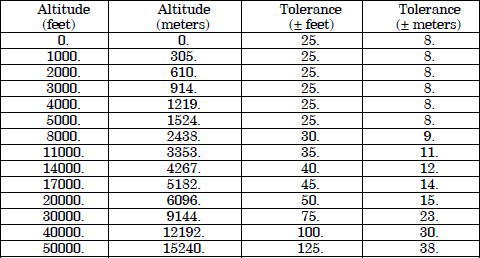
In Table 6.2, we see that the absolute error for the indicated altitude (Indicated_Alt) provided by an ADC installed in an aircraft (AC) should be less than 25 ft when this aircraft is actually situated between 0 and 5,000 ft, for this indicator to be considered to comply with the airworthiness requirement FAR 29.1303(b). In other words, expressed in terms of PBR, we will have:

PBR₁: when AC.Alt ∈[0.0, 5000.0[→| ADC.Indicated _Alt | AC.Alt | ≤ 25.0 ft

Moreover, we see that this PBR alone is not sufficient to cover the whole flight domain (beyond 5,000 ft). Thus, we will introduce the following additional PBRs to be able to cover the whole domain considered by the standard:

PBR₂: when AC.Alt ∈[5,000.0, 8,000.0 ft[ → |ADC.Indicated_Alt - AC.Alt | ≤ 30.0 ft

PBR₃: when AC.Alt ∈[8,000.0, 11,000.0 ft[ → |ADC.Indicated_Alt - AC.Alt | ≤ 35.0 ft

PBR₄: when AC.Alt ∈[11,000.0, 14,000.0[ → |ADC.Indicated_Alt - AC.Alt | ≤ 40.0 ft

PBR₅: when AC.Alt ∈[14,000.0, 17,000.0[→ |ADC.Indicated_Alt - AC.Alt | ≤ 45.0 ft

PBR₆: when AC.Alt ∈[17,000.0, 20,000.0[→ |ADC.Indicated_Alt - AC.Alt | ≤ 50.0 ft

PBR₇: when AC.Alt ∈[20,000.0, 30,000.0[→ |ADC.Indicated_Alt - AC.Alt | ≤ 75.0 ft

PBR₈: when AC.Alt ∈[30,000.0, 40,000.0[→ |ADC.Indicated_Alt - AC.Alt | ≤ 100.0 ft

PBR₉: when AC.Alt ∈[40,000.0, 40,000.0[→ |ADC.Indicated_Alt - AC.Alt | ≤ 125.0 ft

We can, therefore, interpret the airworthiness requirement FAR 29.1303(b) as the conjunction of nine PBRs above (PBR _{FAR 29.1303(b)} = PBR₁∧.. ∧PBR₉); it is wise to have the following assumption, which assumes that the AC flight domain is situated between 0 and 50,000 ft (above the mean sea level (MSL)), which can be written:

ASSUMP₀: AC.Alt ∈[0.0, 50000.0[

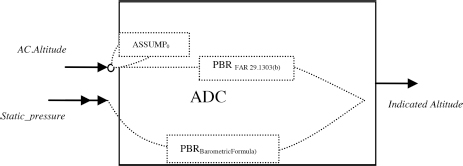
Figure 6.5. Some PBRs linking inputs and outputs of an air data computer

Here, we have shown that a requirement can be interpreted as a conjunction of PBRs.

Similarly, we can also specify how indicated altitude has to be computed from static pressure by using a body of knowledge on atmospheric data such as the Manual of the ICAO Standard Atmosphere [ICA 64] to express the following PBR_{BarometricFormula}:

PBR_{BarometricFormula}: when AC.Alt ∈[0.11km[→

|ADC.Indicated_Alt-
BarometricFormula(AC.Pressure) | ≤ 25.0 with

BarometricFormula(AC.Pressure)

6.6.2. Example 2: FAR29.951(a) Fuel systems - General

We can also consider another airworthiness requirement that is also subject to interpretation. This is the general requirement FAR29.951(a). We have chosen this as it takes place in the domain of continuous systems (fluids).

FAR 29.951 Fuel systems - General

a) Each fuel system shall be constructed and arranged to ensure a flow of fuel at a rate and pressure established for proper engine and auxiliary power unit functioning under any likely operating conditions, including the maneuvers for which certification is requested and during which the engine or auxiliary power unit is permitted to be in operation.

This requirement includes helicopter fuel systems subject to FAR 29. It refers to an essential property of an aircraft fuel system, namely to supply fuel to the associated engine. The statement “the fuel system shall supply fuel to the engine” it not itself a requirement, since a system that does not supply fuel cannot be called a fuel system (here, the functional requirement concept is useless). The requirements are the modalities according to which the system shall supply the fuel, as requirement FAR 29.951 indicates, to provide fuel (continuously) to the assigned engine, at the flow rate and pressure required by the engine, under all operation conditions (including authorized operations), and throughout the whole duration of the authorized operation.

PBR_FuelFeed: when Ctrl= Feeding ∧ c in Operation_conditions ∧ t in Operation_time→ |Fuel_System.Fuel_Rate&Pressure (c,t)- Engine_Demand(t)| ≤ tol

This requirement is read as follows: when the system is in feeding mode, and the operation conditions (altitude, temperature, etc.) remain in a defined domain, and the operation time does not exceed a defined time, then the fuel system shall supply the continuous flow of fuel required by the engine with an acceptable pressure level.

Figure 6.6. Some PBRs linking inputs and outputs of an aircraft fuel systemE

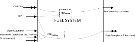
We can also introduce a requirement for the filling of the system with fuel, which links the quantity of fuel contained in the system and the quantity of fuel supplied when the system is in refueling mode.

PBR_Refuel: when Control= Refueling→ | |Fuel_System.Fuel_Quantity (t_f) Fuel_System.Fuel_Quantity (t_i) | - _ti∫tf Fuel_Flow(t)dt | ≤ tol

In other words, when the system is in refueling mode, the difference between the contained quantity at the end of filling and that contained at the start shall be equal (within a stated tolerance, to account for acceptable losses) to the quantity supplied to the system.

Additional requirements can be added to these two requirements, for example, a maximum refueling time and others about the fuel gauging accuracy, reliability, etc.

To conclude on the interpretation of TBRs, note that many TBRs keep implicit the object to which they relate. Also, many system specifications contain requirements that do not relate to itself, but to the associated processes such as the development process (for example, “software assurance level of the SAS⁷ shall be A in accordance with DO-178C” means that the software development process of the SAS software will satisfy the objectives required by DO-178C for the level A) or the system operating process (such as weight and balance requirements that the operator will respect when cargo is loaded on board an aircraft).

6.7. Conclusion: specification models and concurrent assertions

A system is usually represented graphically in the form of a rectangle with inputs and outputs as shown in Figure 6.7.

Figure 6.7. Canonical graphical representation of a system

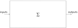
This summary representation of a system appeals to our imagination but it disregards several facts:

First, this representation does not always, unlike a schematic representation, provide a true physical image of the system’s physical bonds. Thus, the feed line (physical link) that links the fuel system to an engine (in a schematic representation) is represented here as an input (for example, an requested flow rate which is a first charachetristic of the fuel line.) and an output (for example, a fuel pressure exerted which is the second charachetristic of the same fuel line- input and output provide the two variables of a power bond.). In fact, what is shown in this canonical representation is a sequence of causes and effects. Represented to the left of the rectangle are the causes (inputs), whereas to the right are the effects (outputs), visible effects of a system, consequences of actions suffered by the system and its own activity [THO 75].

Second, most systems have a memory (like human beings) and the outputs at a given moment in time not only depend on the inputs at that moment but also on all previous inputs (in the case of causal systems).

To account for this, there are two possibilities:

For the specification model of a type of systems, the second point of view has been adopted rather than the first; the temporal approach is much more intuitive and natural than the frequency approach to most engineers. This causes the specification model of a system (that makes the inputs, observable states and outputs) to be not in biunivocal correspondence with the inputs and outputs of physical systems as shown below. If the inputs and outputs of the specification model correspond to the inputs and outputs of specific physical systems by regrouping inputs and outputs⁸, the observable states of the specification model correspond to internal states that have been “externalized” for modeling purposes and to make the model observable.

In this context, the specification model of one type of systems would be equivalent to the conjunction of two PBRs, the first specifying the intended state of the type of systems, as in the state equation, and the second specifying the intended outputs of one type system, as in the output equation.

The specification model of a type Σ of systems can be represented graphically as follows:

Figure 6.8. System specification model. For a color version of this figure, see www.iste.co.uk/micouin/MBSE.zip

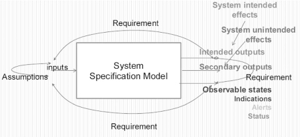
When a statement O.P(C,D) (for [when C] → val(O.P) ∈ D), condition C is first assessed:

During the simulation process, the assertions that make up a specification model of a type Σ of systems are assessed in parallel. This means that, at each simulation cycle, all assumptions (requirements or assumptions) that shall be assessed, because the associated triggering events have occurred, are effectively evaluated and the concurrent assessment results are plotted by the simulator. In one cycle, one or several requirements or assumptions may be breached, indicating either an error in the specification or an error in the design, as we will study later on in Chapters 8 and 9.

1 The initial spark of the PBR theory partially comes from the chapter 3 of “System Requirements Analysis”, written by Jeffery O Grady, and on an intellectual inheritance from B language, invented by J.R Abrial.

2 In this section, we use the term “collection” rather than the term “set” to highlight the dynamic character of a collection: a collection may be empty at a given moment such as the collection of aircraft corresponding to an ongoing definition, then to a variable number of copies when the first specimens, corresponding to a given definition, exit the assembly lines and put into operation.

3 According to the ISO15288 standard, the Design Office is an enabling system for the system of interest (p. 55).

4 A typology, strictly speaking, is a mathematical partition of a set E, that is to say any element of E belongs to one and only one partition for each level of the typology.

5 These are a ransom paid to pragmatism and consensualism.

6 In the past, other standards have prevailed (SAE-AS 362).

7 SAS: stabilization augmentation system.

8 Thus, a shaft bond involves both an input (for example, rotational speed of the shaft) and an output (transmitted torque), whereas an electrical signal can be a twisted pair of electric cables.