Laplacian Operator

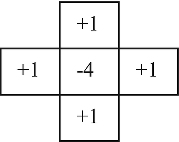
An efficient method of edge detection is that of zero crossing of the Laplacian. The Laplacian operator is defined in mathematics as the sum of the second partial derivatives:

Lap(F(x, y)) = ∇²F(x, y) = ∂²F/∂x² + ∂²F/∂y².

Because a digital image is not differentiable, it is necessary to replace the derivatives by finite differences.

Definition 1: The expression D₁(x, Δx, F) = F(x + Δx) - F(x) is called the first difference of F(x) with respect to x and with the increment Δx.

Definition 2: The expression D_n(x, Δx, F) = D₁(x, Δx, D_n-1(x, F(x)) with n > 1 is called the nth difference of F(x) with respect to x and with the increment Δx. The second partial differences with respect to x and y are equal to

D₂(x, Δx, F) = F(x – Δx, y) - 2·F(x, y) + F(x + Δx, y)

D₂(y, Δy, F) = F(x, y – Δy) - 2·F(x, y) + F(x, y + Δy)

and the finite Laplacian with Δx = Δy = 1 is equal to

∇²F(x, y) = F(x – 1, y) + F(x + 1, y) - 4·F(x, y) + F(x, y – 1) + F(x, y + 1).

It can be calculated in digital images with the filter shown in Figure 6-2.

An application of this filter to a digital image with the gray values F(x, y) yields the following value:

∇²F(x, y) = F(x – 1, y) + F(x + 1, y) - 4·F(x, y) + F(x, y – 1) + F(x, y + 1)(6.1)

Equation 6.1 can be rewritten as follows:

∇²F(x, y) = F(x – 1, y) + F(x + 1, y) + F(x, y – 1) + F(x, y) + F(x, y + 1) - 5·F(x, y)

= 5·M(x, y) - 5·F(x, y) = 5·(M(x, y) - F(x, y))(6.2)

where M(x, y) is the mean value of F(x, y) of the five pixels in the neighborhood of the pixel with coordinates (x, y). It is also possible to calculate the finite Laplacian in the pixel P = (x, y) by subtracting the gray value of P from the local mean value in the neighborhood of P. It is appropriate to use the fast averaging filter (Chapter 2) when using a greater neighborhood.

The Method of Zero Crossing

The method of zero crossing is based on detecting locations where the Laplacian changes its sign. Consider the cross-section through a row of a digital grayscale image shown in Figure 6-3.

The Laplacian has positive values on one side of an edge and negative values on its other side. The absolute values of Laplacian near the edge are great as compared with its values on locations far away from the edge. It is more practical using the negative value of Laplacian—that is, the value (F(x, y) – mean value) instead of the value (mean value – F(x, y))—because these values are greater at greater gray values.

Locations at which the Laplacian changes its sign are called zero crossings. Some of these locations correspond to the location of the edge. A zero crossing always lies between two pixels. These indications of the location of an edge are therefore always quite thin.

Are Zero Crossings of Laplacian Closed Curves?

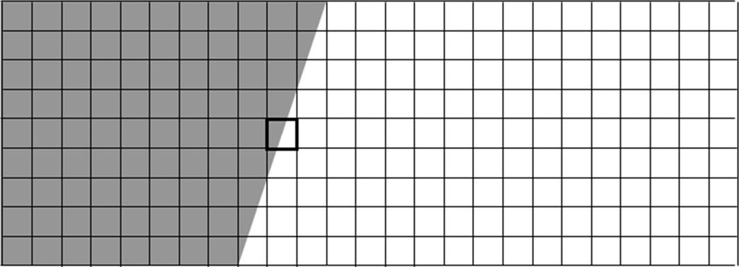
One advantage of the Laplacian put forward in some textbooks on image processing is that the edges produced by Laplacian are always closed lines. However, this is true only if we threshold the values of Laplacian; for example, if we replace the positive values of the Laplacian by 1 and the negative ones by 0. The fact that the boundaries of sets of pixels with the value 1 in such an image are closed curves is, however, the advantage of binary images and not that of Laplacian. Such edges are shown in Figure 6-4b. Most edges in an image of the Laplacian binarized with a threshold equal to 0 are irrelevant.

As you can see, the overwhelming majority of the white lines in Figure 6-4b are completely meaningless and cannot be used as edges. These are the so-called irrelevant zero crossings.

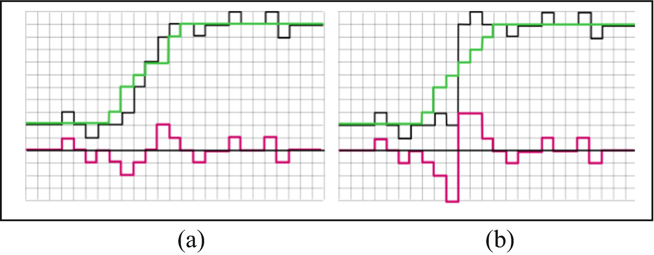
Figure 6-5 shows an explanation for the irrelevant zero crossings of the Laplacian. The black lines shows the gray values of the original image. The green line represents the local mean value of the gray values, and the red line is the Laplacian. Red arrows show the irrelevant zero crossings. The values of the Laplacian at these locations are small, whereas at the relevant crossing the absolute value of the Laplacian is great.

We explain in the next section how to eliminate the irrelevant zero crossings.

How to Eliminate Irrelevant Crossings

Irrelevant crossings can be distinguished from the relevant ones by means of two thresholds: Only transitions from a Laplacian value greater than a positive threshold to a Laplacian value less than a negative threshold should be recognized as relevant edges. Most irrelevant edges disappear, but some relevant ones are interrupted due to the noise in the image. The image should be filtered to reduce the noise, for example, with the simplest averaging filter (Chapter 2). The image should be filtered two times: with a small and with a greater gliding window. The differences between these two filtered images can then be regarded as a good approximation of the Laplacian.

Consider Figure 6-6b, which shows as a blue line the gray values in one row of the image. The Laplacian values are shown as a green line. The black line is the x axis; red lines show the thresholds used to distinguish between relevant and irrelevant zero crossings. A zero crossing is relevant if it lies between two such pixels that one of them has a Laplacian value greater than the positive threshold and the other pixel has a Laplacian value less than the negative threshold.

Figure 6-7 explains how the irrelevant zero crossings can be eliminated.

Noise Reduction Before Using the Laplacian

When using the averaging filter for noise reduction, the edges become blurred. As a result, the difference between the positive and negative values of Laplacian becomes small; Laplacian values change gradually. This makes it difficult to distinguish between relevant and irrelevant zero crossings. We suggest using the sigma filter (Chapter 2) instead of averaging with a small window. Then the edges remain precipitous; the absolute amounts of the Laplacian become larger.

Black lines in Figure 6-8a show the gray values filtered with averaging with a small window. In Figure 6-8b, the black line represent the gray values filtered with the sigma filter. For both, green lines represent the local mean values with the greater window and red lines show the Laplacian values.

Blur During the Digitization and Extreme Value Filter

Even an ideal edge can become somewhat blurred during the digitization of an image. The reason for this is that the boundary between a light and a dark area in an image projected to the set of light-sensitive elements (e.g., CCD, charge-coupled devices, electronic light sensors used in various devices including digital cameras) can fall occasionally near the center of an element, as shown in Figure 6-9.

This element obtains a light amount, which we call the middle value, lying between the values that are proper for the light and dark areas. The corresponding pixel is located in the middle of the edge and the Laplacian obtains a small value or even a zero value. A gap in the detected edge occurs, as illustrated in Figure 6-10.

Consider an example of edges detected by the Laplacian zero crossing method (threshold = 10) after using the sigma filter and the extreme value filter. Figure 6-11 shows the gray values of the original image (Figure 6-11a) and the images after successive steps of processing the image with the filters: the image processed with the sigma filter (Figure 6-11b), with the extreme value filter (Figure 6-11c), and the Laplacian with edges (Figure 6-11d). Positive Laplacian values are shown in red, negative values in blue, and zero crossings as white lines.

As you can see, the edge detection is rather successful. However, there are some gaps in the edges as explained in the next section.

Fundamental Errors of the Method of Zero Crossing in the Laplacian

Laplacian has a fundamental property that the sequences of its zero crossings must have gaps in the neighborhood of points where three or four sequences meet. Figure 6-12 provides an example. Figure 6-12 shows an artificial image (a), the edges detected by the method of zero crossing (b), the desired ideal edges (c), and the values of the sign of the Laplacian (d). The red pixels are the pixels with positive values of the Laplacian and the blue pixels are those with negative values. Zero crossings are shown in Figure 6-12d as white lines.

Notice the missing pieces of the edges occurring due to fundamental errors in Figure 6-12 marked by green arrows. These are considered fundamental errors because it is impossible to eliminate them. These errors occur because the Laplacian is the difference between the local mean and the actual gray value. A zero crossing lies between a pixel with a positive value and one with a negative value of the Laplacian. One of these pixels has a gray value greater than the local mean and the other one a gray value less than the local mean. If, however, there are more than two different gray values in the gliding window, then the local mean can lie only between two of gray values. There can be no zero crossing for the third gray value. The edge therefore has a gap. Due to these gaps, the edges produced by means of Laplacian zero crossings contain no crotches.

These errors are very important because edges are often used to produce polygons representing boundaries of areas with a constant color. Missing crotches make these polygons incomplete, as they do not describe the boundaries of regions correctly.