
In computer vision, image segmentation is the process of partitioning a digital image into multiple segments (sets of pixels, also known as super-pixels). The goal of segmentation is to simplify and/or change the representation of an image into something that is more meaningful and easier to analyze.[1][2] Image segmentation is typically used to locate objects and boundaries (lines, curves, etc.) in images. More precisely, image segmentation is the process of assigning a label to every pixel in an image such that pixels with the same label share certain characteristics.
There are in the scientific literature a giant number of publications on methods of segmentation. Let us, however, remember that any thresholded image can be considered a segmented one. Also a quantized image, where all the gray values or colors are subdivided in a relatively small number of groups with a single color assigned to all pixels of a group, can be considered segmented. The difficulty of the segmentation problem consists only in the possibility of defining meaningful segments; that is, segments that are meaningful from the point of view of human perception. For example, a segmentation for which we can say, “This segment is a house, this one is the street, this one is a car, and so on,” would be a meaningful segmentation. As far as I know, developing a meaningful segmentation is an unsolved problem. We consider in this section segmentation by quantizing the colors of an image into a small number of groups optimally representing the colors of the image.
Segmentation by Quantizing the Colors
Quantizing the colors is the well-known method of compressing color images: Color information is not directly carried by the image pixel data, but is stored in a separate piece of data called a palette, an array of color elements. Every element in the array represents a color, indexed by its position within the array. The image pixels do not contain the full specification of the color, but only its index in the palette. This is the well-known method of producing indexed 8-bit images.
Our method consists of producing a palette optimal for the concrete image. For this purpose we have developed the method MakePalette described in Chapter 8 and successfully used in the project WFcompressPal.
Connected Components
We suppose that the segments should be connected subsets of pixels. Connectedness is a topological notion, whereas classical topology considers mostly infinite sets of points where each neighborhood of a point contains an infinite number of points. Classical topology is not applicable to digital images because they are finite.
The notion of connectedness is also used in graph theory. It is possible to consider a digital image as a graph with vertices that are the pixels and an edge of the graph connects any two adjacent pixels. A path is a sequence of pixels in which each pixel besides one at the beginning and one at the end is incident to exactly two adjacent pixels.
It is well known (refer e.g. to Hazewinkel, (2001)) that in an undirected graph, an unordered pair of vertices {x, y} is called connected if a path leads from x to y. Otherwise, the unordered pair is called disconnected.
A connected graph is an undirected graph in which every unordered pair of vertices in the graph is connected. Otherwise, it is called a disconnected graph.

The connectedness paradox: (a) the four adjacency, and (b) the eight adjacency
Rosenfeld (1970) suggested considering the eight adjacency for black pixels and the four adjacency for white pixels in a binary image. This suggestion solves the problem in the case of binary images, but it is not applicable to multicolor images. The only solution of the connectedness paradox for multicolored images I know of consists of considering a digital image as a cell complex as described in Chapter 7. The connectedness can then be defined correctly and free from paradoxes by means of the EquNaLi rule (refer to Kovalevsky (1989)) specified below.
Two pixels with coordinates (x, y) and (x + 1, y + 1) or (x, y) and (x – 1, y + 1) make up a diagonal pair. A pair of eight adjacent pixels is defined as connected in the theory of ACCs if both pixels have the same color and the lower dimensional cell (one- or zero-dimensional) lying between them also has this color. Naturally, it makes little sense to speak of color of lower dimensional cells because their area is zero. However, it is necessary to use this notion to consistently define connectedness in digital images. To avoid using the notion of colors of low-dimensional cells we suggest replacing color by label when the label of a pixel is equal to its color.
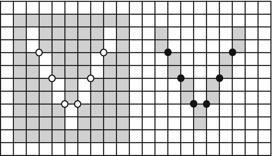
White and black V-shaped regions in one image, both connected due to applying the EquNaLi rule
The EquNaLi rule for two-dimensional images states that a one-dimensional cell always receives the greatest label (lighter color) of two principal (i.e., two-dimensional) cells incident to it.
If the 2 × 2 neighborhood of c0 contains exactly one diagonal pair of pixels with equal labels (Equ), then c0 receives this label. If there is more than one such pair but only one of them belongs to a narrow (Na) stripe, then c0 receives the label of the narrow stripe. Otherwise c0 receives the maximum; that is, the lighter (Li) label (i.e., the greater label) of the pixels in the neighborhood of c0.
The latter case corresponds to the cases when the neighborhood of c0 contains no diagonal pair with equal labels or it contains more than one such pair and more than one of them belong to a narrow stripe.
To decide whether a diagonal pair in the neighborhood of c0 belongs to a narrow stripe it is necessary to scan an array of 4 × 4 = 16 pixels with c0 in the middle and to count the labels corresponding to both diagonals. The smallest count indicates the narrow stripe. Examples of other efficient membership rules can be found in Kovalevsky (1989).
It is important for the analysis of segmented images to find and to distinguish all connected components of the image. The problem is finding the maximum connected subsets of the image, each subset containing pixels of a constant color. Then it is necessary to number the components and to assign to each pixel the number of the component it belongs to. Let us call the assigned number a label.
A subset S of pixels of some certain color is called connected if for any two pixels of S there exists a sequence of neighboring pixels in S containing these two pixels. We consider the EquNaLi neighborhood.
To find and to label the components, an image must contain a relatively small number of colors. Otherwise each pixel of a color image could be a maximum connected component. Segmented images mostly satisfy the condition of possessing a small number of colors.
The naive approach involves scanning the image row by row and assigning to each pixel that has no adjacent pixels of the same color in the already scanned subset the next unused label. If the next pixel has in the already scanned subset adjacent pixels of the same color and they have different labels, the smallest of these different labels is assigned to the pixel. All pixels of the already scanned subset having one of these different labels must obtain this smallest label. The replacement might affect in the worst case up to height2/2 pixels, where height is the number of rows in the image. The total number of replacements after the whole image is scanned could then be on the order of height3/2. This number can be very large, so the naive approach is not practical. An efficient method of labeling the pixels of one component is the well-known and widely used method of graph traversal.
The Graph Traversal Algorithm and Its Code
Let us consider now the graph traversal approach. The image is regarded as a graph and the pixels are regarded as vertices. Two vertices are connected by an edge of the graph if the corresponding pixels have equal values (e.g., colors) and are adjacent. The adjacency relation can be the four or eight adjacency. It is easily recognized that the components of the graph correspond exactly to the desired components of the image.
There are at least two well-known methods of traversing all vertices of a component of a graph: the depth-first search and the breadth-first search algorithms. They are rather similar to each other, and we consider here only the breadth-first search. This algorithm was used in our projects containing suppression of impulse noise (Chapter 2). We describe it here in a little more detail.
- 1.
Set the number NC of the components to zero.
- 2.
Take any unlabeled vertex V, increase NC, label V with the value NC and put V into the queue. The vertex V is the “seed” of a new component having the index NC.
- 3.Repeat the following instructions, while the queue is not empty:
- 3.1.
Take the first vertex W from the queue.
- 3.2.
Test each neighbor N of W. If N is labeled, ignore it; otherwise label N with NC and put it into the queue.
- 3.1.
- 4.
When the queue is empty, then the component NC is already labeled.
Proceed with Step 2 to find the seed of the next component until all vertices are labeled.
Let us describe the pseudo-code of this algorithm. Given a multivalued array Image[] of N elements and the methods Neighb(i,m) and Adjacent(i,k), the first one returns the index of the mth neighbor of the ith element. The second one returns TRUE if the ith element is adjacent to the kth one and FALSE otherwise. As a result of the labeling each element gets the label of the connected component to which it belongs. The label is saved in an array Label[], which has the same size as Image[]. We assume that all methods have access to the arrays Image and Label and to their size N.
The Pseudo-Code of the Breadth-First Algorithm
End of the Algorithm
The value Max_n is in this case the maximal possible number of all neighbors of an element of the image regardless of whether it was already visited or not. It is equal to 8. It is necessary to provide the queue data structure with the methods PutIntoQueue(i), GetFromQueue(), and QueueNotEmpty(). The last method returns TRUE if the queue is not empty; otherwise it returns FALSE.
This algorithm labels all pixels of a component containing the starting pixel. To label all components of an image it is necessary to choose the next starting pixel among those not labeled as belonging to an already processed component. This must be repeated until all pixels of the image are labeled.
The Approach of Equivalence Classes
There is another approach to the problem of labeling connected components, that of equivalent classes (EC), which considers labeling all components of an image simultaneously. One of the earliest publications about the approach of EC is that by Rosenfeld and Pfalz (1966). The idea of this algorithm in the case of a two-dimensional image proceeds as follows. The algorithm scans the image row by row two times. It investigates during the first scan for each pixel P the set S of all already visited pixels adjacent to P according to the four or eight adjacency and having the same color as P. If there are no such pixels, then P gets the next unused label. Otherwise P gets the smallest label (the set of labels must be ordered; integers are mostly employed as labels) of the pixels in S. Simultaneously the algorithm declares all labels of the pixels of S as equivalent to the smallest label. For this purpose the algorithm employs an equivalence table, where each column corresponds to one of the employed labels. Equivalent labels are stored in the elements of the column.
When the image has been completely scanned, a special algorithm processes the table and determines the classes of equivalent labels. Each class is represented by the smallest of equivalent labels. The table is rearranged in such a way that in the column corresponding to each label, the label of the class remains. During the second scan each label in the image is replaced by that of the class.
One of the drawbacks of this algorithm is the difficulty of estimating a priori the necessary size of the equivalence table. Kovalevsky (1990) developed an improved version of the EC approach, independent of Gallert and Fisher (1964), called the root method . It employs an array L of labels, which has the same number of elements as the number of pixels in the obtained image. This is a substitute for the equivalence table. To explain the idea of the improvement we consider first the simplest case of a two-dimensional binary image, although the algorithm is applicable also in the case of multivalued and multidimensional images without essential changes.
The suggested method is based on the following idea. Each pixel of the image has a corresponding element of the array L of labels. Let us call it the label of the pixel. The array L must be of such a type that it is possible to save in its elements the index x + width*y of each pixel of the image (the type integer is sufficient for images of any size). If a component contains a pixel with a label that is equal to the index of this pixel, then this label is called the root of the component.
At the start of the algorithm each element of the array L corresponding to the pixel (x, y) is set equal to the index x+width*y where width is the number of columns of the image. Thus at the start each pixel is considered a component.
The algorithm scans the image row by row. If a pixel has in the previously scanned area no adjacent pixel of the same color, then the pixel retains its label. If, however, the next pixel P has adjacent pixels of the same color among the already visited pixels and they have different labels, this means that these pixels belong to different previously discovered components having different roots. These different components must be united into a single component. It is necessary for this purpose to find the roots of these components and to set all these roots and the label of P equal to the smallest root. It is important to notice that only the roots are changed, not the values of the labels of the pixels adjacent to P. Labels of the pixels will be changed in the second scan. This is the reason this method is so fast. All components that meet at the running pixel get the same root and they are merged into a single component. The labels that are not roots remain unchanged. In the worst case previously mentioned, the replacement could affect only width/2 pixels.
After the first scan, the label of each pixel is pointing to a pixel of the same component with a smaller label. Thus there is a sequence of ever smaller labels ending with the root of the component. During the second scan all labels are replaced by subsequent integer numbers.
The connectedness of subsets must be defined by an adjacency relation. This can be a well-known (n, m) adjacency that is defined only for binary images, or an adjacency relation based on the membership of the cells of lower dimensions in the subsets defined by the method EquNaLi.

Example of an image with four colors having as many components as the number of pixels
If it is known that the number of used labels is smaller than size, then an array L with a smaller number of bits per element can be sufficient for applying the method using an equivalence table. However, this is not important in the case of modern computers, which have ample memory. So, for example, an array of the data type int on a modern computer with a 32-bit processor can be employed for images containing up to 232 elements. Thus a two-dimensional image can have a size of 65,536 × 65,536 pixels and a three-dimensional image a size of 2,048 × 2,048 × 1,024 voxels.
Let us return to the algorithm. It scans the image row by row and investigates for each pixel P the set S of already visited pixels adjacent to P. If there are in S pixels of the same color as that of P and they have different labels, then the algorithm finds the smallest root label of these pixels and assigns it to P and to the roots of all pixels of S. Thus all components that meet each other at the running pixel obtain the same root and are merged into a single component. The labels of pixels that are not roots remain unchanged. In the worst case of a single component, the replacement can affect only width/2 pixels.
Each pixel belongs after the first scan to a path leading to the root of its component. During the second scan the labels of the roots and all other pixels are replaced by subsequent integer numbers.
A simple two-dimensional example is presented in Figure 9-4. Given is a two-dimensional binary array Image[N] of N = 16 pixels. Two pixels of the dark foreground are adjacent if and only if they have a common incident 1-cell (four adjacency), whereas pixels of the light background are adjacent if they have any common incident cell (eight adjacency). At the start of the algorithm the labels of all pixels are equal to their indexes (numbers from 0–15 in Figure 9-4a). The pixels with the indexes 0 and 1 have no adjacent pixels of the same color among the pixels visited before. Their labels 0 and 1 remain unchanged. They are the roots. The pixel with the index 2 has the adjacent pixel 1, which has a root of 1. Thus label 2 is replaced by 1. Label 3 remains unchanged after the scanning of the first row. The labels of all pixels are changed according to the preceding rule until the last pixel 15 is reached. This pixel is adjacent to pixels 11 and 14. The label of pixel 11 is pointing to root 3; that of pixel 14 is pointing to pixel 0, which is also a root. Label 0 is smaller than 3. Therefore the label of the root 3 becomes replaced by the smaller label 0 (Figure 9-4b).
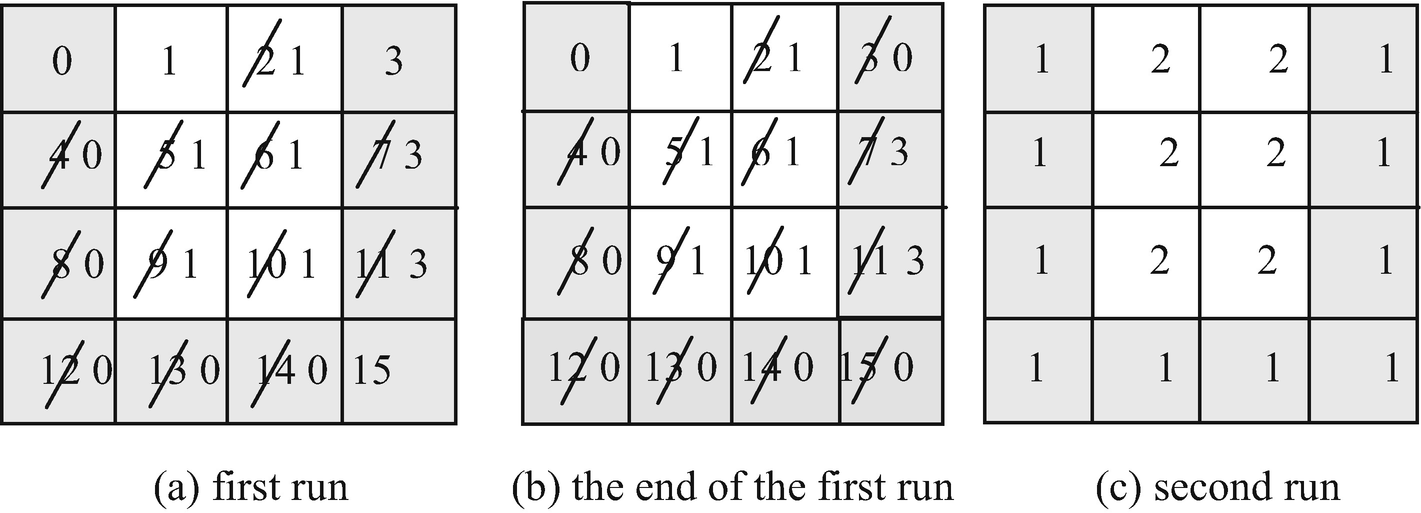
Illustration of the algorithm for labeling connected components
The Pseudo-Code of the Root Algorithm
This algorithm can be applied to an image either in a combinatorial or in a standard grid. In a combinatorial grid, where the incidence relation of two cells is defined by their combinatorial coordinates, it is sufficient to assign a value (a color) from the set of values of the pixels to each cell of any dimension. Two incident cells having the same value are adjacent and will be assigned to the same component. In a standard grid a method must be given that specifies which grid elements in the neighborhood of a given element e are adjacent to e and thus must be assigned to the same component if they have the same value. In our earlier simple two-dimensional example, we have employed the four adjacency of the foreground pixels and the eight adjacency of the background pixels. In general, the adjacency of principal cells of an n-dimensional complex must be specified by rules specifying the membership of cells of lower dimensions (e.g., by a rule similar to the EquNaLi rule), as the well-known (m, n) adjacency is not applicable to multivalued images. We consider here the pseudo-code for the case of the standard grid .
Given is a multivalued array Image[] of N elements and the methods Neighb(i,m) and Adjacent(i,k). The first one returns the index of the mth neighbor of the ith element, and the second one returns TRUE if the ith element is adjacent to the kth one. Otherwise it return FALSE. In the two-dimensional case this can be a method implementing the EquNaLi rule. As a result of the labeling, each element obtains the label of the connected component to which it belongs. The label is saved in another array Label[].
The array Label[N] must be the same size as Image[N]. Each element of Label must have at least log2N bits, where N is the number of elements of Image, and must be initialized by its own index:
for(i = 1; i < N; i++) Label[i] = i.
To make the pseudo-code simpler, we assume that all methods have access to the arrays Image and Label and to their size N.
In the first loop of the algorithm each element of Image gets a label pointing to the root of its component. The value Max_n is the maximum possible number of adjacent elements of an element (pixel or voxel) that have already been visited. It is easily recognized that Max_n is equal to (3d - 1)/2, where d is the dimension of the image. For example, in the two-dimensional case, Max_n is equal to 4 and in the three-dimensional case it is equal to 13.
The subroutine SetEqu(i,k) (its pseudo-code is seen next) compares the indexes of the roots of the elements i and k with each other and sets the label of the root with the greater index equal to the smaller index. Thus both roots belong to the same component. The method Root(k) returns the last value in the sequence of indexes where the first index k is that of the given element, the next one is the value of Label[k], and so on, until Label[k] becomes equal to k. The subroutine SecondRun() replaces the value of Label[k] by the value of a component counter or by the root of k depending on whether Label[k] is equal to k or not.
The Project WFsegmentAndComp
We have developed a Windows Forms project WFsegmentAndComp segmenting an image and labeling the pixels of its connected components.
It is possible to perform the segmentation in two ways: either by clustering the colors into a relatively small number (e.g., 20) of clusters and assigning to each cluster the average color of all pixels belonging to the cluster, or by converting the color image to a grayscale image, subdividing the full range [0, 255] of the gray values to a small number of intervals, and assigning to each interval the average gray value. The conversion does not cause a loss of information because the labels of the connected components are relatively great numbers having no relation to the colors of the original colors: The set of pixels having a certain color can consist of many components, with each component having another label.
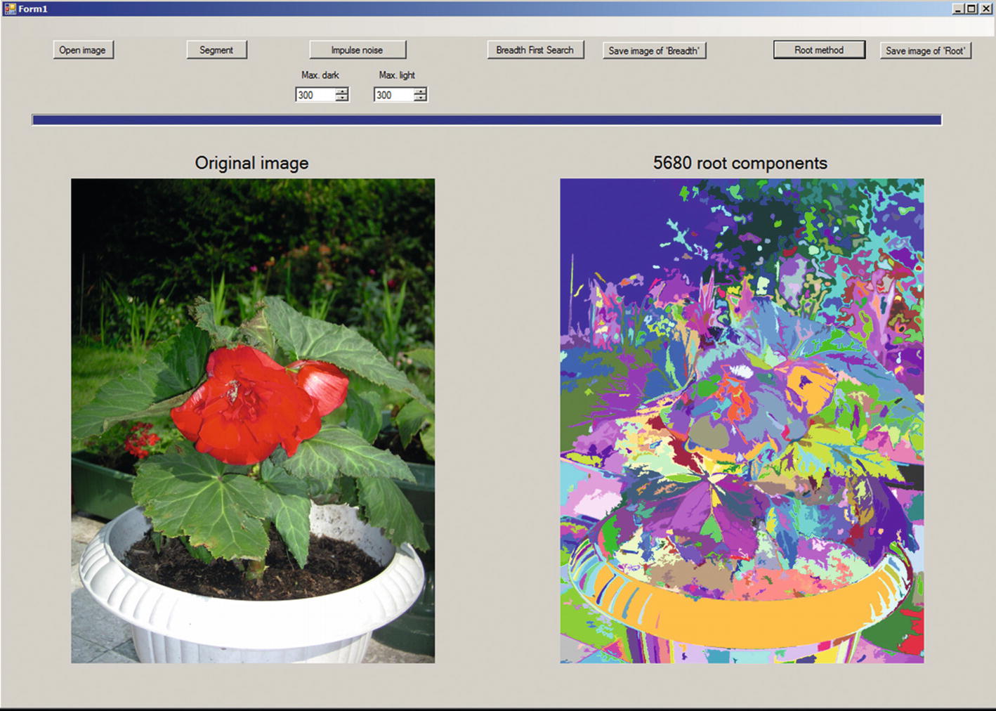
Form of the project WFsegmentAndComp
When the user clicks Open image, he or she can choose an image to be opened. The image will be presented in the left-hand picture box, and five work images will be defined.
The user should then click the next button, Segment. The original image will be converted to a grayscale image. The gray values will be divided by 24 and the integer result of division will be multiplied by 24. In this way the new gray values become multiples of 24 and the scale of the gray values is quantized into 256/24 + 1 = 11 intervals. The segmented image is presented in the right-right picture box.
It is known from experience that the number of components, even of a segmented image, is very large. Among the components are many consisting of a single pixel or few pixels. Such components are of no interest for image analysis. To reduce the number of small components we have decided to suppress impulse noise of the segmented image. This merges many small spots of a certain gray level with the surrounding area and reduces the number of small components.
The user can choose the maximum sizes of dark and light spots to be deleted and click Impulse noise. The image with deleted dark and light spots will be presented instead of the segmented image.
Then the user can click either Breadth First Search or Root method. The labeled images will be shown in false colors; that is, with an artificial palette containing 256 colors. The index of the palette is equal to dividing the label by 256.
The code for suppressing impulse noise was presented in Chapter 2.
Here we present the code of for breadth-first search used for labeling connected components of the segmented image. As already mentioned, this algorithm processes the pixels of one component containing the start pixel. To process all components of the image we have developed the method LabelC, which scans the image and tests whether each pixel is labeled. If it is not, then it is a starting pixel for the next component and the method Breadth_First_Search is called.
As one can see, the method is very simple: it scans all pixels of the image and checks whether the actual pixel is already labeled. If it is not, then the method Breadth_First_Search is called.
The bitmap BreadthBmp shows the components in false colors.
The user can save the image with the labeled components as a color image by clicking Save image of ‘Breadth’.
The image RootIm of the class CImageComp contains the labels of the components and the palette. As in the case of Breadth_First_Search, the methods MakePalette and LabToBitmap are called to make the labels visible. The image RootIm is transformed to the bitmap RootBmp and the latter is displayed in the right-hand picture box. Then the user can save this image by clicking Save image of ‘Root’.
Conclusion
The time complexity of both the root algorithm and the breadth-first algorithm is linear in the number of the elements of the image. Both algorithms can be applied to images of any dimension provided the adjacency relation is defined.
Numerous experiments performed by the author have shown that the runtime of both the root algorithm and the breadth-first algorithm is almost equal. The advantage of the root algorithm is that it tests each element of the image whether it is already labeled or not (3d - 1)/2 times with d equal to 2 or to 3 being the dimension of the image, whereas the breadth-first algorithm tests it 3d times, which is approximately two times more. The breadth-first algorithm can be directly employed to label only a single component containing a given element of the image, whereas the root algorithm must label all components simultaneously.