Two More Random Walks

15.1 Brownian Motion

Perhaps the best known drunkard’s walk is called Brownian motion, named after the Scottish botanist Robert Brown (1773–1858) who, in 1827, observed (under a microscope) the chaotic motion of tiny grains of pollen suspended in water drops. (This motion had been previously noted by others, but Brown took the next step of publishing what he saw in an 1828 paper in the Philosophical Magazine.) This motion exhibits a number of interesting physical characteristics: the higher the temperature and the smaller the suspended particle the more rapid the motion, while the more viscous the medium the slower the motion; the motions of even very close neighboring particles are independent of each other; the past behavior of a suspended particle has no bearing on its future behavior; and the likelihood of motion in a particular direction, at any instant of time, is the same for all directions. Figure 15.1 shows a typical (very kinky) 1,000-step two-dimensional path of a particle executing Brownian motion in a plane.1 The beginning and the end of the path are marked with a B and an E, respectively.

Figure 15.1. Typical path of a particle executing Brownian motion in a plane.

Today, because of the work by the German-born physicist Albert Einstein (1879–1955) in a series of papers2 published between 1905 and 1908 applying statistical mechanics to the question of Brownian motion, we understand that it is due to the random molecular bombardment experienced by the suspended particles. Brownian motion is, in fact, strong macroscopic experimental evidence for the reality of molecules, and therefore of atoms. Experiments done shortly after Einstein’s theoretical studies that confirmed the theory would earn the French physicist Jean Perrin (1870–1942) the 1926 Nobel Prize in Physics. Some years before that, in the early 1920s, the American mathematician Norbert Wiener (1894–1964) made a deep analysis of the mathematics of Brownian motion, studying in particular what is going on in the limit of a particle moving in steps separated by vanishingly small time intervals. In that limit, Brownian motion becomes what mathematicians call a Wiener stochastic process, a concept of great continuing interest to modern physicists, mathematicians, and electrical engineers.

In particular, a “Wiener walk” is a continuous curve in space that, at almost every point, has no direction. Such “infinitely kinky” curves were known to mathematicians before Wiener’s work,3 but they were what mathematicians like to call pathological, and what other people would say are simply made up, extremely weird curves that are purposely weird just to show the extremes of what mathematics will allow. Wiener’s work showed how such a strange thing could occur, in a natural way, in a physical context. In this discussion I’ll not go anywhere nearly as deep as Wiener did, but there is a very pretty, elementary way of showing how time can be directly introduced into the probabilistic mathematical description of one-dimensional Brownian motion: it is the incorporation of time that makes a random process a stochastic process.

Our random walk will be much like Ross’s mosquito walk in the previous discussion, that is, equally likely, independent steps of length δs, back and forth along the x-axis (δs = l/2 is Ross’s walk). After N such steps, the particle, which has to be somewhere, could be at any one of the x-axis points -Nδs, (-N+1)δs,…,-δs,0, δs, (N-1)δs, Nδs. To be precise, to be at the point with x-axis value mδs, it is necessary that (N+m)/2 of the steps—it doesn’t matter which ones—were in the positive direction and the other (N — m)/2 steps were in the negative direction. (Notice that m can be even only if N is even, and that m can be odd only if N is odd.) Since the total number of all possible, equally likely left/right step sequences is 2^N, and since the number of sequences for which (N — m)/2 steps are in the negative direction is then the probability the particle is at x = m δs after N steps is

We can express (15.1) in a much different, and actually far more informative way, as follows. Expanding the binomial coefficient in the numerator, we have

From Stirling’s asymptotic formula for factorials,4 that is from

we have

So, taking the natural logarithm of (15.1) and using Stirling’s approximation, we have

Suppose now that we limit ourselves to the cases where m << N, that is, we will concentrate our attention on the probabilities that the particle has not wandered out nearly as far as it might possibly wander from its starting point at x = 0. Even though Stirling’s approximation is just asymptotic, the fact that the numerator of (15.1) contains the ratio of factorials means our final approximation to P (m <<, N)will be pretty accurate even in the absolute sense if m << N. I’ll show you how that works numerically in just a bit. Now, using the power series expansion approximation

we have

Similarly,

So, for m <<

If you multiply this all out you’ll find that a lot of terms cancel; in addition, making the final approximation that (since N >> m) results in or, at last

We can numerically compare, for any given N and all possible m, the approximate (15.2) to the exact (15.1) to see how much damage all of our approximations have caused. Suppose, for example, that N= 12 (and so m = 0, ±2, ±4,…, ±12 are the particle location possibilities). Then,

m	(15.1)-exact	(15.2)-approximation
0	0.2256	0.2303
2	0.1934	0.1950
4	0.1208	0.1183
6	0.0537	0.0514
8	0.0161	0.0160
10	0.0029	0.0036
12	0.00024	0.00057

As you can see, (15.2) is actually a pretty good approximation, even for m ≈ N.

To finish our analysis, I’ll next express the x-axis coordinate of our particle as x = mδs. Thus, m = x/δs, and so (15.2) becomes

In addition, suppose we now consider intervals along the x-axis of length δx such that δx >> δs; this means that there are numerous points within a δx interval at which the Brownian particle might be after N steps. Note carefully—both δx and δs are small, but δs is very small! Then the probability the particle is somewhere in the interval (x,x+δx) is

where the sum is over all possible points on the x-axis where the particle could be located. To evaluate the sum, we need only make the following two observations:

With these two observations, we can write (15.4) as

or

For our last step in this analysis, which in fact is the crucial step that introduces time, let’s suppose that the particle makes n steps per unit time. Then, starting from t = 0, the particle has made N = nt steps at time t. This lets us write (15.5) as

or, if we define the so-called diffusion coefficient5 then we can write

as the probability the particle is in the interval (x, x+δx) at time t. Since a probability is the product of a probability density and an interval (δx), that is W(x, t) = f_X(x,t)δx where f_X(x,t) is a pdf, we see from (15.6) that

is the pdf6 that describes the location on the x-axis of a particle executing one-dimensional Brownian motion.7 The pdf of (15.7) contains time and, obviously, it changes with time. Random processes that have pdf’s that do not change with time are said to be stationary (in time). So, the one-dimensional Brownian motion of a particle is a nonstationary random process, and it is a favorite of probability textbook authors looking for an example to illustrate that concept.

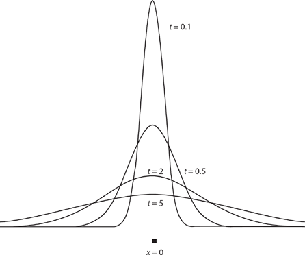
Figure 15.2. Gaussian pdfs for one-dimensional Brownian motion.

For a given value of time, the pdf of (15.7) is the well-known bell-shaped Gaussian curve, named for the great German mathematician Carl Friedrich Gauss (1777–1855), who studied it long before anyone had any idea it would occur in the theory of Brownian motion. For all non-negative values of t the pdf is symmetrical about x = 0. For values of t only slightly positive the bell-shaped pdf is tall and narrow, as the particle has not yet had enough time to wander very far from its starting point, but as time increases the bell-shaped pdf broadens and becomes less spiked. This reflects the fact that the total area under the pdf curve, which is the probability the particle is somewhere, is always unity. Figure 15.2 shows the relative shapes and sizes of (15.7) for four values of time. Notice that these curves clearly illustrate Karl Pearson’s comment, in his second Nature letter (see the previous discussion), that at all times “in open country the most probable place to find a drunken man who is at all capable of keeping on his feet is somewhere near his starting point!” That is, for intervals of fixed width δx, the one that has the largest probability of containing the particle is always the one centered on x = 0.

15.2 Shrinking Walks

In the random walks so far considered, the walker could, in the limit as the number of steps increases without bound, be found arbitrarily far from the starting point—the origin—of the walk. This is because the length of each step has been, so far, a constant. There is another interesting class of random walks, however, that is forever confined to a finite region of space even as the number of steps increases without limit. These are walks in which every step is shorter than the previous one. In particular, I’ll discuss here what is called a one-dimensional geometric walk, in which the nth step has length sⁿ, where n = 0 is the first step and s is a positive number less than one. So, the lengths of the first four steps, for example, are 1, s, s², and s³. I’ll take the steps as independent and equally likely to be in either direction along the x-axis. That is, if ε_n = ±1 with equal probability, then the location of the walker at the end of N steps is

The maximum distance of the walker from the origin occurs when ε_n = ±1 for all n:

which is a geometric series (hence the name of the walk), easily summed, to give

and so, even as N → ∞, the location of the walker is restricted to an interval of finite width 2/(1 — s) centered on the origin. For example, if s = 0.6, then the resulting geometric walk will always be somewhere in an interval of length 5 centered on the origin, no matter how many steps long the walk may be.

As a variation on this sort of random walk, we could reinterpret the ε_nas equally likely to be 0 or +1, which physically represents a walk that, on the nth decision, either stays at the current location (ε_n = 0) or moves one step to the right (ε_n = 1). There is never a step to the left. Such a walk drifts to the right, but it too, of course, will always be confined to a finite interval, in this case to 0 < x < 1/(1 — s), 0 < s < 1. Making ε_n= 0 or − 1 would give a walk drifting to the left.

Walks with nonconstant step size have been known to mathematicians since the 1930s, but in recent years they have also attracted the attention of physicists. For example, the authors of a paper8 published in 2000 encountered such a walk during a “study of the state reduction (collapse) in multiple position or momentum observations of a quantum-mechanical particle.” Well, that sounds pretty deep to me—I have no intention of jumping into that pool!—and my only point here is that walks with a changing (in this case, decreasing) step size can have physical significance. In fact, the other extreme, of an increasing step size, can occur in physics as well. For example, in a 1992 paper9 it is shown that a particle executing Brownian motion in a fluid with a linear shear flow (imagine a wide river in which water flows ever faster downstream the farther out from one bank you move) performs a random walk with a step size that increases linearly with each new step. The authors call this walk a “stretched walk.”

In the rest of this section I’ll follow the lead of an even more recent (2004) paper that presents a fascinating mathematical discussion of geometric walks.10 In particular, the authors, whom I’ll refer to as K&R, were interested in the probability density functions of the distance x of the walker from the origin after an infinity of steps. That is, suppose we define the pdf for that distance as a function of the number of steps, and the step size, by fX,s(x, N). Then the question asked by K&R is, what happens as N → ∞ that is, what is

In general, this is not an easy question. But K&R do offer some quite interesting partial answers. For example,

(1) if s > ½ the subset of the x-axis where f_X,s (x) is non-zero is a Cantor set, that is, is fractal (which means, in practical terms, that we can not plot fX,S (x) for s < ½);

(2) if s = ½, then f_X,s (x) is uniform; and

(3) if ½ ≤ s < 1, then f_X,s(x) is continuous.

These results are formally derived by K&R, but we can get an intuitive idea of what is going on with some Monte Carlo simulation, an approach K&R themselves use in the beginning of their paper. For example, suppose we take a look at the case of a right-drifting shrinking random walk with s = 1/2. We can’t, of course, simulate such walks with an infinite number of steps, but just to get some idea of what happens, let’s pick N= 29 steps (as do K&R), simulate 2,000,000 such random walks (K&R looked at 100,000,000 random walks), and record where the walk is at the end of the last step. Using the same sort of coding approach I used in the previous discussion, such a simulation produced Figure 15.3, and it does indeed suggest that in the limit N → ∞ f_x,s (x) is uniform over 0 < x < 2 when s = 1/2 (remember, the simulation gives an estimate of f_X,s(x, 29)). The nature of fX,s(x) changes dramatically, however, for s ≠ 1/2; for example, Figure 15.4 shows the result of simulating a twenty-nine-step random walk for s = (and as you’ll soon see, that particular, perhaps curious-looking value for s was not chosen at random).

Before saying more about , let me make one final comment about the s = 1/2 case. K&R show, using some high-powered math (Fourier transforms), how to formally derive f_X,s(x) for the values of s = 2^-1/m where m is a positive integer. The very first value of m, m = 1, gives s = 1/2, and the formal result is a uniform pdf. If you are willing to settle for a less inclusive proof, however, one that works just for the single case of s = 1/2, there is a surprisingly simple proof of uniformity. If we put s = 1/2 in (15.8), then

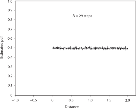
Figure 15.3. Shrinking walk for s = 0.5.

Interpreting all the ε_i as either 0 or 1 (a drifting walk), this expression for the location of the walk at the end of the Nth step is simply an N-bit binary number in the interval . All possible combinations of values for all the ε_i give all possible N-step walks, with the numbers and the walks in a one-to-one correspondence. Since the binary numbers are uniformly distributed over the interval —I hope the uniformity is obvious!—then the walk lengths are uniform, too. In Figure 15.3 I used N = 29, and so there are a total of 2²⁹ = 536,870,912 such walks, while the simulation code that produced Figure 15.3 randomly examined just 2,000,000 walks. The wiggles you see in that figure are statistical sampling effects caused by looking at only a very small fraction of all possible twenty-nine-step walks.

Sampling error is just the first of our concerns with studying geometric walks by Monte Carlo simulation. Equally troublesome is that, as N increases, the step size becomes so small it eventually gets lost in roundoff error. There is a beautiful way, for one particular value of s, at least, to avoid this new problem. K&R give a broad overview of the approach, as follows, for walks that have both left and right moving steps:

However, we need a method that provides the end point location without any loss of accuracy to resolve the fine details of [f_x,s (x,N)]. … For large N, the accuracy in the position of a walk is necessarily lost by roundoff errors if we attempt to evaluate the sum for the end point location directly.

To solve this problem for the particular value of K&R conclude this part of their paper with the following somewhat enigmatic (in my opinion) words:

Pretty intriguing stuff, alright, but what does it mean? K&R don’t provide any of the details of their “reduction”, and absent is any discussion of A and B, that is, they don’t provide us with formulas with which to calculate A and B. What follows is my reconstruction of what they did, and (in my opinion) what K&R did is pretty darn clever!

To start, consider the second order difference equation

which is of course the famous Fibonacci equation, named after the Italian mathematician Leonardo Pisano (circa 1170–1250), also known by the sobriquet Fibonacci.11 Just as we can often solve differential equations by assuming an exponential solution, we can often solve difference equations by assuming a power solution. That is, let’s assume

where c and k are some yet to be determined non-zero constants. Then, substituting this into (15.9), we have

or

This quadratic is easily solved to give

So, in general,

where, for complete generality, I’ve used a different c for each of the two k’s. Using the given conditions u(0) = u(1) = 1, it is not difficult to show that the constants c1 and c2 are

Thus,

or, at last,

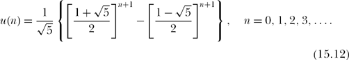
As K&R indicate, the Fibonacci number F_n = F(n) satisies (15.9), except that we normally start the indexing at n = 1 rather than at n = 0. All we need do, then, is replace n + 1 in the exponents of (15.12) with n = 1, 2, 3,…, and so

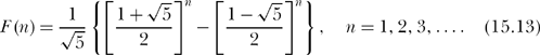
The Fibonacci numbers are, of course, all integers (1, 1, 2, 3, 5, 8, 13, …), and I have always found it amazing that for every single one of the infinity of positive integer values of n, an expression like (15.13), with all of its irrational , produces an integer.12

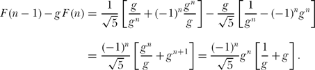
Next, let’s set g = 1/k₁, where we pick the value of k > 0 so that g > 0. Then, from (15.10), we have

or

which, you’ll recall, K&R call “the defining equation.” The physical interpretation of (15.15), which can be written as 1 — g — g² = 0, is that g is that value of step size such that an initial step to the right (the “1”), followed by a second step to the left (the “—g”), followed by a third step to the left (the “—g²”), returns the walk exactly to the origin. Notice that returning exactly to the origin in three steps is impossible with a constant step size.

It is easy to verify that

and that

Inserting these two results into (15.13), we have

or

Since we know from (15.14) that

then multiplying through by g gives

Using (15.17) in (15.16) gives

And from (15.18) we have

or

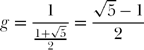
Consider now F (n — 1) — g F(n). That is, from (15.19) and (15.18) we can write

Using (15.17), we know that

and so

As we showed earlier,

and so

and so

Inserting this into (15.20) we have

or

which is K&R’s “remarkably simple formula.”

Now we can calculate A and B. We have, onceagain, from(15.8), that the location of the end of our walk is at (with s = g)

That is, just to be quite clear, x_N is the endpoint of a geometric walk with N steps with a step size factor of g (with a first step of length ε₀ =±1 with equal probability). So, writing x_N in detail, and using (15.21),

And this is, indeed, as K&R say, “the much simplier form A+Bg. That is, in the particular random geometric walk with s = g (called by K&R the “golden walk, for the obvious reason), with both left-and right-moving steps, the endpoint of the walk after N steps is

where

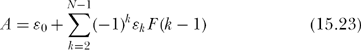
and

where all the ε’s = ±1 with equal probability and the F’s are the Fibonacci numbers of (15.13).

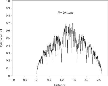
Figure 15.4. Shrinking walk for

To see how (15.23) and (15.24) work, let’s take a look, in two different ways, at golden walks with twenty-one steps. There are 2²¹ =2,097,152 such walks. First, as with Figure 15.4 (golden walks with twenty-nine steps), we can randomly simulate a lot of twenty-one-step walks and from them generate an estimate of the pdf for the location of the endpoints, that is, an estimate for f_{x, g} (x, 21). And second, using (15.23) and (15.24), we can compute the endpoints of each and every one of the 2²¹ walks and thus arrive at the exact f_{x, g} (x,21). This second approach does not use a random number generator. The upper plot of Figure 15.5 shows the result of 2,097,152 simulated walks (this allows for the possibility of each and every one of the possible twenty-one-step walks to be generated). The lower plot in Figure 15.5 shows the result of directly computing the endpoint of each and every possible walk. The spatial resolution in both plots is 10-², that is, there are 524 subintervals with width 0.01 in the interval The two plots are to the eye at least identical.

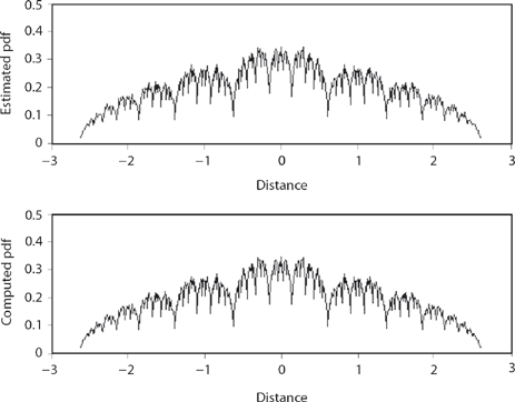
Figure 15.5. Simulated and computed golden walks.

CP. P15.1:

In the discussion on geometric walks, we’ve looked only at shrinking walks. What does the pdf of a stretched walk look like? As a start to answering this, you are to write a Monte Carlo simulation of a stretched random walk with s = 1.01. That is, the step sizes are 1, 1.01, 1.01², 1.01³, …. Write the code for a simulation that estimates the pdf of the endpoint location of a twenty-one-step walk, with left- and right-moving steps equally likely. Plot the pdf with a spatial resolution of 10^-2. That is, since the maximum distance from the origin (the walk’s starting point) is

then the required number of subintervals (into which the individual endpoints of the simulated walks are placed) is . It’s always a good idea to have some idea of the nature of a solution before arriving at that solution, just as a partial check. Can you see, right now, that the value of the pdf at x = 0 must be zero? That is, it is impossible for this stretched walk to ever return to its starting point. Make sure your simulation agrees with this. If it does, that does not mean the simulation is correct, but if it doesn’t agree, that does mean the simulation is incorrect!

Notes and References

1. Figure 15.1 was created by a MATLAB program I wrote for my book, Duelling Idiots and Other Probability Puzzlers (Princeton, N.J.: Princeton University Press, 2000 [corrected ed. 2002]). It’s called brownian.m, and you can find the code on p. 210 of that book or on the press’s math Web site (the code is available for download, for free) at http://press.princeton.edu/titles/6914.html. Superficially similar random behavior had been observed long before Brown’s time. A half-century before Jesus, the Roman philosopher Lucretius wrote the following in Book 2 of his poem, De rerum natura (On the Nature of Things):

Some writers have claimed this is an early description of Brownian motion, but I suspect it has more to do with sunlight unequally heating the air and the resulting macroscopic thermal air currents rather than with the microscopic, molecular origin of true Brownian motion.

2. You can read, in English, these beautiful papers by Albert Einstein in Investigations on the Theory of the Brownian Movement (New York: Dover, 1956 [originally published in 1926]).

3. See, for example, my book, When Least Is Best (Princeton, N.J.: Princeton University Press, 2004 [corrected ed. 2007], pp. 40–45).

4. An asymptotic expansion has the property that while the expansion has an unbounded absolute error, its relative error approaches zero. That is, if E(n)is an asymptotic expansion for some function f(n), then

but

For f(n) = n!, the decrease in the relative error of Stirling’s approximation, as n increases, is remarkably fast. The approximations for 1! = 1, 2!= 2, and 5! = 120 are 0.9221, 1.919, and 118.019, respectively (the percentage errors are 8%, 4%, and 2%, respectively), while for 10! = 3,628,800 the approximation is 3,598,600 (a relative error of just 0.8%). For more on this, see lan Tweddle, “Approximating n! Historical Origins and Error Analysis” (American Journal of Physics, June 1984, pp. 487–488), as well as the essay “Stirling’s formula!” in the book by N. David Mermin, Boojums All the Way Through: Commuicating Science in a Prosaic Age (Cambridge: Cambridge University Press, 1990).

5. This is a mathematical definition. The diffusion coefficient is physically a simple function of two universal constants, the gas constant and Avogadro’s number (both well-known to students of high school chemistry), the absolute temperature, and the viscosity of the suspension medium. While known today as a theoretician, Einstein was not just a symbol pusher; the physics of D appears in much detail in his papers on Brownian motion (see note 2).

6. If fx(x, t) is a pdf, then it must be true, for any given t > 0, that since this is the certain probability that the particle is somewhere on the x-axis. And it certainly must be somewhere! That is, it must be true that This is of course a purely mathematical assertion (with a clear physical interpretation), and so the question arises: can we mathematically prove that this is so? I still have a strong memory of discussing this very integral as a first-year graduate student at Caltech (1962–1963) with a fellow student in a course in which it came up in lecture one day. The professor just assumed everybody knew the value of the integral, and when I expressed surprise after class at that assumption, my fellow student (who, unlike me, had done his undergraduate work at Caltech), expressed surprise at my surprise. I was told every Techie alive knew that particular integral by the end of their freshman year. While I had no reason to doubt that claim, I soon realized that the main goal of my classmate was to wage a bit of psychological warfare on somebody who had come to Caltech from someplace else. Still, I also quickly realized that in this matter he was right—this integral is something every undergraduate in physics, engineering, and mathematics should indeed know how to do. Here’s how. Write the integral

Since x is just a dummy integration variable, it is also true that

Thus, multiplying these two expression together, we get

That is, I² is the integral of the function over the entire infinite xy plane, where dxdy is the differential area in rectangular coordinates. Now, change variables to polar coordinates r and θ, where of course x²+y² = r² and the differential area is rdrdθ. To cover the infinite plane we have 0 ≤ r ≤ π and 0 <2π. (For how to make coordinate transformations like this in general, see any good advanced calculus book and look in its index for a discussion of Jacobian transformations.) So,

Thus, and the assertion is indeed correct. Is that slick, or what?

7. The density of (15.7) is perfectly well defined for all t > 0, but at t = 0 it does seem to behave badly. Since the particle is at x = 0 at t = 0 (by definition, with absolute certainty), then we must have

where δ(x) is Dirac’s famous impulse or delta function, often written by engineers and physicists as

such that (see note 6 again)

Mathematicians are generally appalled at this sort of “engineer’s math,” but I believe it is okay to write

and then to talk of how δ(x) behaves inside an integral. You can find much more on Dirac’s impulse in my book, Dr. Euler’s Fabulous Formula (Princeton, N.J.: Princeton University Press, 2006, pp. 188–206).

8. A. C. de la Torre et al., “Random Walk With An Exponentially Varying Step” (Physical Review E, December 2000, pp. 7748–7754).

9. E. Ben-Naim, S. Redner, and D. ben-Avraham, “Bimodal Diffusion in Power-law Shear Flows” (Physical Review A, May 15, 1992, pp. 7207–7213).

10. P. L. Krapivsky and S. Redner, “Random Walks With Shrinking Steps” (American Journal of Physics, May 2004, pp. 591–598). This paper (which repeats much of the mathematics in the earlier paper I cited in note 8), while totally mathematical in nature, does mention another physics appearance of a variable-step random walk (in spectroscopy), in which the size of the nth step is 1/n³. The maximum distance such a walk can be found from the origin is then which gives us yet another appearance of the zeta function in physics (see Discussion 7).

11. See my book, An Imaginary Tale: The Story of (Princeton, N.J.: Princeton University Press, 1998, [corrected ed. 2007], p. 249).

12. Perhaps almost as amazing is that it wasn’t until four centuries after Fibonacci that the French mathematician Albert Girard (1595–1632) first wrote the definition of the Fibonacci sequence in the form given by (15.9). And it took two more centuries for the French mathematician Jacques Binet (1786–1856) to discover (in 1834) the solution to (15.9) given in (15.13). There is evidence, however, that (15.13) was known a century earlier to the French-born mathematician Abraham de Moivre (1667–1754), who did all his great mathematical work after emigrating to England in 1688.