Random Walks

14.1 Ronald Ross and the Flight of Mosquitoes

In September 1904, at the International Congress of Arts and Science in St. Louis, Sir Ronald Ross (1857–1932) gave an interesting talk (reprinted a year later in Science)1 on how to mathematically model the spread of mosquitoes from a breeding pool. As the vectors of such devastating diseases as yellow fever and malaria, understanding how these insects migrate was an important practical problem of the day. Yellow fever in particular had some years before laid waste to the French effort to build a Panama Canal. Ross was not a mathematician by training—he was a British medical doctor who had received the 1902 Nobel Prize in Medicine for his work on malaria—but his simple mathematical analysis is still of interest.

Ross prepared his audience for the mathematics to come with these words:

He had earlier hinted at the probabilistic mathematics he was about to introduce when he said,

Ross began by imagining that the life of a mosquito can be divided into n stages; during each stage the insect can fly a total distance of l. He further imagined, for mathematical simplicity, that while individual insects each begins its life by flying away from its birthplace at a random angle (which is almost surely different for each mosquito), once picked that angle remains fixed for each mosquito. (Fixing our attention now on one mosquito in particular, we lose no generality in imagining its line of flight is along the x-axis. Multiple mosquitoes, taken together, will of course be distributed over a two-dimensional plane.) During each of its stages of life, imagine that our mosquito decides, twice, at random, whether to fly “forward” or “backward” by a distance of l/2. Ross took the forward and backward choices to be independent and equally likely (each with probability 1/2). So, for example, if t = 0 is the time of birth of our mosquito, then at time t = 1 the insect is either at x = l/2 with probability 1/2 or at x =—1/2 with probability 1/2. At t = 2 the insect is at x = l with probability 1/4, or at x =—l with probability 1/4, or back at x = 0 with probability 1/2. And so on. Since the mosquito makes 2n decisions during its lifetime, the unit of time is simply that lifetime divided by 2n (Ross argued that n could be taken as large as one pleased, and so of course l could be made as small as one pleased). Ross never gave a name to this sequential decision process, but today mathematicians call it a one-dimensional random walk.

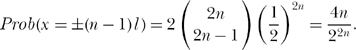
Ross next invoked a very simple combinatorial argument to compute the probabilities the mosquito’s “dead body” would be found at x = 0, x = ±l, x = ±2l,…, x = ±nl, where it should be clear that those are the only locations at which it could be found; that is, since the mosquito makes an even number of flight direction choices (2n), its final location must be an even multiple of l/2. For example, for the mosquito to be at either nl or at—nl, all of its 2n decisions must have been in the same direction. Thus,

For the mosquito to be at either (n − 1)l or at — (n − 1)l, all but one of its 2 n decisions must have been in the same direction, with one additional decision in the opposite direction. Thus,

For the mosquito to be at either (n − 2)l or at — (n − 2)l, all but two of its 2 n decisions must have been in the same direction, with two additional decisions in the opposite direction. Thus,

And so on, until we get to the x = 0 case. Then precisely half of the mosquito’s decisions are in one direction and the other half are in the reverse direction. Thus,

To give a specific numerical example of these expressions, Ross imagined that the initial total number of mosquitoes is 1,024 (he set n = 5 in 2²ⁿ). Then the expected number of mosquitoes reaching the various possible distances from the starting point is just the numerators of the above probability expressions. That is,

Distance from the breeding pool	Number of dead mosquitoes
0	252
l	420
2l	240
3l	90
4l	20
5l	2

Ross wrote of these numbers,

Ross thought so much of this observation that he elevated it to a general principle: “The law here enunciated may, perhaps, be called the centripetal law of wandering. It ordains that when living units wander from a given point guided only by chance they will always tend to revert to that point.” As far as I know, mathematicians and physicists have not adopted Ross’s somewhat grandiose “Newtonian” terminology.

14.2 Karl Pearson Formulates a Famous Problem

In the summer of 1905, almost a year after Ross’s address, the eminent English statistician Karl Pearson (1857–1936) wrote a letter to the British science journal Nature in which he asked for help on a mathematical problem. The problem was a sophisticated version of Ross’s mosquito migration problem and one Ross himself had earlier asked for help on from Pearson. The letter is short, and so, because of its historical importance, I will quote it here in full:2

This letter is historically important because it gave the name to one of the most beautiful subjects in probability theory (itself considered by many to be one of the most beautiful areas of mathematics3), the theory of the random walk (in this case, a true two-dimensional random walk, unlike Ross’s mosquito walk, which, despite appearances, is really just one-dimensional).

A reply4 was published in the very next issue of Nature as a letter signed only as Rayleigh. No more identification was needed, in fact, as the author was known to all as the brilliant mathematical and experimental physicist John William Strutt (1842–1919), who sat in the House of Lords as Lord Rayleigh and who just the previous year had received the Nobel Prize in Physics for his discovery of argon. (Rayleigh was one of those rare individuals who could have been legitimately awarded multiple Nobel Prizes many of his other discoveries, as well.) Rayleigh’s letter was even shorter than Pearson’s:

This probability5 is of the form f_r(r)dr, where f_r(r) is called a probability density function (pdf):

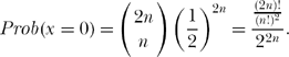
is famous today as Rayleigh’s pdf (see Figure 14.1 for the case of n = 6, for example—this is not “very great,” but you’ll soon see why I picked this value), and there isn’t a modern textbook on introductory probability theory that doesn’t devote a fair amount of space to deriving and discussing its many applications.6

As a testament to the very rapid mail delivery in those long ago days, Pearson’s reply7 to Rayleigh appeared in yet the very next issue of Nature. Pearson’s letter is quite interesting, as comments in it will motivate much of what appears later in this discussion. So, quoting Pearson again:

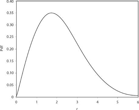
Figure 14.1. Rayleigh’s pdf for n = 6.

(And so, in that last sentence, we see yet another example of the “mutual embrace” of mathematics and physics that I mentioned in the Preface.) Pearson’s letter continues:

Pearson’s last sentence makes Ross’s point that most of a large number of mosquitoes will die near their breeding pool. It also contributed the colorful alternative name of drunkard’s walk to the random walk process, a name you can find in many modern probability books.

I’ll return to the second letter from Pearson later in this discussion, but first let me remark that while Ross clearly described a one-dimensional random walk, and while Pearson gave the name random walk to a more sophisticated version of Ross’s problem, they were definitely not the first to touch on such questions.9 In 1865, for example, the Irish-born mathematician Morgan Crofton (1826–1915) proposed the following pretty little problem:

Crofton is remembered today as one of the early developers of geometric probability, and his solution shows how nicely the elementary concepts of that subject handle this question with ease. The answer is that the probability of returning to the river is 1/4—can you see how to calculate that? (I’ll show you the solution at the end of this section, but see if you can figure out where the 1/4 comes from before reading the solution.)

A few years later, in 1873, the English mathematician J.W.L. Glaisher (1848–1928) posed a question very much more like what Pearson would ask thirty-two years later:

Figure 14.2. Crofton’s problem.

Glaisher’s problem, while much more mathematically sophisticated than Crofton’s (and Pearson’s, too), suffered the same fate of both in failing to stimulate additional study.

Okay, have you solved Crofton’s problem? If not, here’s how to do it. After the first day’s journey the traveler could be anywhere on a semicircle centered on his starting point, as shown in Figure 14.2. Now, focus on one possible first day’s journey, shown in the figure as the dashed line at angle θ₁ in the interval 0 to π/2 (θ₁ can actually be anywhere in the interval 0 to π/2, but for now let’s work with 0 to π/2). For that angle, any second angle θ₂ in an interval of width π − 2θ₁ will result in a return to the river (see the figure). Since θ₁ is uniformly distributed from 0 to π, θ₁ is a random variable with probability density fθ₁(θ₁) = 1/π.θ₂ is also a uniform random variable, but over the interval 0 to 2π, and so has probability density fθ₂(θ₂) = 1/2π. So, writing P(return|θ₁ = θ₁) as the so-called conditional probability of returning to the river for the particular angle θ₁, we have

To calculate P(return) we need to integrate out the dependency on θ₁, that is

Since the situation for an initial angle θ₁ in the second quadrant (π/2 ≤ θ₁ ≤ π) is symmetrical with the first quadrant case we just analyzed, our total probability of return is double this, that is,

14.3 Gambler’s Ruin

Drunkard’s walk is but one colorful name given to the one-dimensional random walk. Another, a name that doesn’t even sound like a random walk at all (but is), is gambler’s ruin. This is a favorite of mathematicians as a classroom example, but for us the real reason for its interest is that it can be solved exactly, in analytical form. That will be useful for us when I show you yet another, approximate way to solve random walk problems; we can check how well the approximate solution for gambler’s ruin agrees with the theoretically exact solution. There are numerous variations of gambler’s ruin, but I’ll treat one of the simplest, a version that can be traced back to a problem posed by the French mathematician Blaise Pascal (1623–1662) in 1654.

Suppose two people, A and B, agree to play the following game. Together, initially, they have five one-dollar bills, with three of them A’s and the other two belonging to B. They also have a penny that, when flipped, shows heads with probability p and tails with probability q (with p+q = 1, as we’ll assume landing “on edge” never occurs). A and B start flipping the penny, where we’ll also assume the individual flips are independent of one another. Each time the coin shows heads A gets one of B’s dollar bills, and each time it shows tails A gives one of his dollar bills to B. The game ends when one of them first has all the money. What is the probability A is ruined, that is, loses all of his money to B? This is mathematically equivalent to saying A starts at x = 3, moves right one step on heads and left one step on tails, and then asking what is the probability A’s position becomes x = 0 (A is ruined) before it becomes x = 5 (A wins all of B’s money, and so it is B who is ruined)?

We can solve for the required probability as follows, beginning with this definition:

u(i) = probability A is ruined, given he starts with i dollars. (14.2)

Then the following equations can be immediately written:

(1) u(0) = 1,

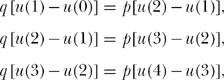
(2) u(1) = qu(0)+pu(2),

(3) u(2) = qu(1)+pu(3),

(4) u(3) = qu(2)+pu(4),

(5) u(4) = qu(3)+pu(5),

(6) u(5) = 0.

The first and last equations are obvious: (1) says A is ruined with certainty if he starts broke, and (6) says A cannot be ruined if he in fact has all the money (five dollars) from the get-go. The other equations are only slightly more subtle. Equation (4), for example, says that the probability A is subsequently ruined (if he starts with three dollars) is the probability he loses on the next flip (probability q) times the probability he is then ruined with his now two dollars, plus the probability he wins on the next flip (probability p) times the probability he is then ruined with his now four dollars. The other equations follows from the same sort of argument.

We can now solve these coupled equations—in particular, for u(3)—using the following clever approach. First, let’s rewrite equations (2) through (5) by multiplying their left-hand sides by 1 (= p+q). Then, rearranging terms, we have

and

If we define

then we have

and

So, remembering that u(0) = 1, we have

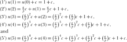
Let’s now assume p ≠ q, that is, that the penny is not a fair coin but rather is biased (the case of a fair coin—when p = q = 1/2, will be separately and easily handled in just a bit). Since u(5) = 0, (5′)says

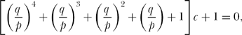
or

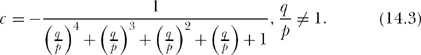
The denominator of (14.3) is a geometric series, easily summed, to give

Now you can see why we took p ≠ q for p = q (14.4) gives the indeterminate result 0/0. We can handle the case of p = qby returning to (5′) and setting p = qthere before summing a geometric series. Then, 5c+1 = u(5) = 0 or,

This special case, of a fair coin, results in the probability solutions

So, the answer to our original question is that, flipping a fair penny, A will be ruined with probability u(3) = 0.4 if he starts with three dollars and B starts with two dollars.

Looking back at (1′) through (4′), you can see, in general, that

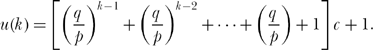
Again, the expression in brackets on the right-hand side is a geometric series, easily summed to give (using (14.4) for the case of an unfair (p ≠ q coin)

or, at last,

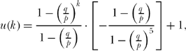
This solution to the gambler’s ruin problem is credited to the Swiss mathematician James Bernoulli (1654–1705); it appears in his Ars Conjectandi (1713). For k = 3,

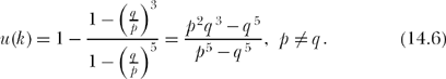
If p= 0.55, for example (and so q = 0.45), we have

as the probability A is ruined if he starts with three dollars and B starts with two dollars, and the penny is not fair. Figure 14.3 shows what u(3) looks like for 0 ≤ p ≤ 1.

14.4 The Monte Carlo Method

The analytical solutions I showed you earlier to Crofton’s problem and the gambler’s ruin problem are elegant and beautiful. But they are also, to different degrees, clever. What if you are not clever? Maybe that’s not a personal concern for these two particular problems, but be absolutely certain in your mind that, no matter how clever you are, there will always be some probabilistic problem that will be beyond your analytical reach. What do you do then? Well, I suppose the first thing to try is to find somebody to help you who is cleverer than you are. But that’s such a depressing task! Here’s another approach—if the problem that has you stumped is based on a well-defined physical process, then try to develop a probabilistic computer simulation of that process. Because of the randomness involved this is called the Monte Carlo approach, and it is now a recognized branch of mathematical physics.10 Let me first show you how it works by applying it to the Crofton and gambler’s ruin problems, and then we’ll return to Pearson’s problem and see what we can do there with some Monte Carlo coding.

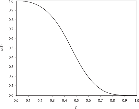
Figure 14.3. Gambler’s ruin.

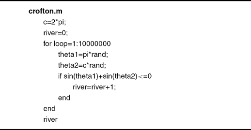
First, Crofton’s problem. The key observation is that, for a return to the river, the net total motion of the traveler in the y-direction (perpendicular to the river) must be nonpositive. The traveler’s motion in the x-direction (parallel to the river) is irrelevant in determining if a return to the river has occurred. In the notation of Figure 14.2, then, the condition for a return is l sin(θ₁) +1 sin(θ₂) ≤ 0, where l is the distance the traveler can journey in a day. The l’s, of course, cancel away, and so we are left with the simple condition of sin(θ₁)+sin(θ₂) ≤ 0 for a return. A very short simulation code is the following (while it is technically MATLAB, I have limited myself to widely used control statements that are found in practically all scientific programming languages; even MATLAB’s rand, which generates numbers uniformly distributed from 0 to 1, is a pretty standard command). This code, called crofton.m, is transparent in its operation; it simply generates ten million random journeys and keeps track of how many of them return to the river. It took me two minutes to write and type it but less than eight seconds for the code to execute on my little home computer. The simulation found that 2,500,964 (the final value of the variable river) returned to the river, giving an estimate of

This is pretty close to the theoretical answer we previously calculated to be 0.25.

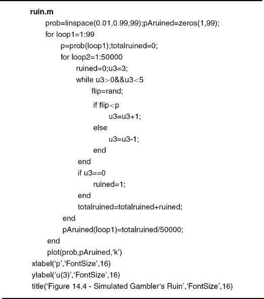
The gambler’s ruin problem is just as easy to simulate, and the MATLAB code ruin.m does the job. It simulates 50,000 games between A and B for each of the uniformly spaced ninety-nine values of p from 0.01 to 0.99, and then creates a plot of u(3) versus p (see Figure 14.4 and then compare it to the theoretical plot in Figure 14.3). In particular, the simulation estimates for p = 0.5 and 0.55, respectively, are u(3) = 0.397 and 0.2911. Both of these Monte Carlo estimates are fairly close to the theoretical values calculated in the previous section (0.4 and 0.2859, respectively). To write ruin.m took about five minutes, but it took only three seconds for the code to execute.

And now, to complete this discussion, let’s go back to Pearson’s plea for help. If personal computers (and a scientific programming language like MATLAB) had been available in 1905, he would have been able to answer his own question, at least numerically, with a Monte Carlo simulation. The surprisingly short code pearson.m is all that is required; after asking for the number of unit-length steps (“stretches” in Pearson’s word) in an individual random walk, the code performs two million such walks (all starting

from the origin) and determines where the walker is at the end of the last step. The squared distance the walker is from the origin—the value of the variable distance2—is stored in the first row of the 2 · 2,000,000 matrix history11, while the actual distance—the square root of distance2—isstoredinthe second row of history.

Figure 14.4. Simulated gambler’s ruin.

We can now use the values stored in history to plot approximations to the probability density functions for the random variables that are the squared distance and the distance of the walker from the origin. As I’ll show you soon, these density functions are easy to calculate exactly for the case of two-step walks (the single case that Pearson said he could do), and we can use those calculations to check the performance of the computer code. Once we are convinced pearson.m is giving us the right results for the two-step walk, we can run it with some confidence for longer walks, walks for which Pearson could not calculate the probability density functions.

This code, unlike either crofton.m or ruin.m, takes advantage of a special MATLAB command, histc (for histogram count). The command N=histc(X,EDGES) creates a vector N that has the same number of elements as does the vector EDGES, such that if EDGES(k) is the value of the kth element of EDGES then N(k) will be the number of elements of the vector X that have values in the interval (EDGES(k), EDGES(k+1)). The elements of EDGES must monotonically increase in value with increasing k. For example, suppose X is the first row vector of history, that is, the values of X are the squared distances of the two million individual walks. Suppose also that EDGES is a row vector whose elements determine the start and stop points (the edges) of 500 subintervals over the interval which a squared distance could occur; for a two-step walk this interval would then of course be (0,4). MATLAB could create EDGES with the command

or, more generally, for a walk of length steps,

Now, if the random variable X has the probability density function pdf(x), and if δx is “sufficiently small” that we can assume the pdf is “constant” over the interval δx, then

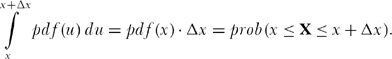
If N(k) is the number of values (out of two million) of the elements of X that fall in the interval (x, x + δx), then

and so

But the length of the subinterval δx is just the length L of the interval in which the values of X could fall (for the distance squared L = steps), and for the distance L = steps), divided by 500 (the number of subintervals). So,

With this explanation, the code pearson.m should now be transparent.

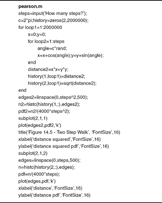
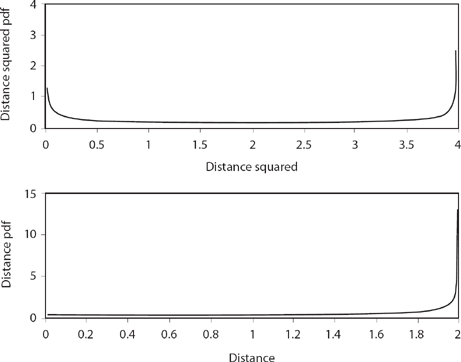
Figure 14.5. Two-step walk.

Figure 14.5 shows the estimated pdfs of the distance and the distance squared random variables for the two-step random walk. Notice that the pdf for the distance squared does indeed have the U-shaped form that Pearson mentions in his second Nature letter, but I have no idea what he meant by “a double U, thus UU, … symmetrical about the centre vertical corresponding to r = 0, but each U itself being asymmetrical.” Further, the U-shaped pdf is for the distance squared, and not for the distance as he requested. The simulation code also gives what Pearson said he was actually after—the pdf for the distance of the walker from the origin—and it is definitely not U-shaped. Are these simulation pdfs in Figure 14.5 correct? let’s calculate them and see.

When the first step (of unit length) is taken we can, with no loss of generality, take the direction as along the positive x-axis. Then, the second step of unit length leads to the geometry of Figure 14.6, with é as a random variable uniformly distributed from 0 to 20; R is a random variable representing the distance of the walker from the origin. From the law of cosines we have the distance squared as

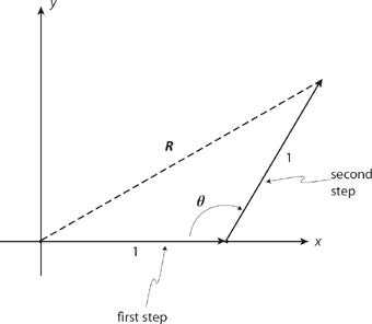
Figure 14.6. The geometry of the two-step walk.

where I’ve written Z = R². To find the pdf of Z, we’ll first find the distribution of Z and then differentiate (see note 6 again). Thus, if Z is the distance squared random variable that takes on values z, we have the distribution

Looking at Figure 14.7 we see that, in the overall interval for θof 0 to 2π, there are two subintervals (labeled a and b) in which cos(θ) . By symmetry the lengths of a and b are equal, and since θ is uniformly distributed these two subintervals have equal probability. So,

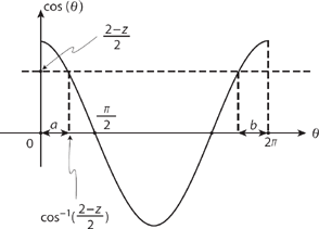
Figure 14.7. Calculating the distribution function for the distance squared of the two-step walk.

The pdf of Z (the distance-squared) is the derivative of the distribution and so

or, using the well-known formula for the derivative of the inverse cosine (look in any good math handbook or calculus textbook, or just derive it for yourself—it’s easy to do), and doing a line or two of easy algebra, we have the pdf for the distance squared as

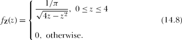
Notice that , and also that the minimum value for f_z(z) occurs when z = 2 and so min f_z(z) = 1/2π = 0.1592. That is, the pdf of the distance squared is shaped like a U, just as Pearson said and as the simulation code pearson.m confirms. Further, the simulation gives a minimum value for the pdf as 0.1586 (the curve in Figure 14.5 is hard to read with accuracy, but a direct examination of the elements of the simulation’s pdf2 vector is easy to do).

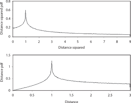
Figure 14.8. Three-step walk.

To calculate the pdf of the distance random variable R, which takes on values r, we have

or, by the same symmetry argument used before,

And so the pdf of R is

or

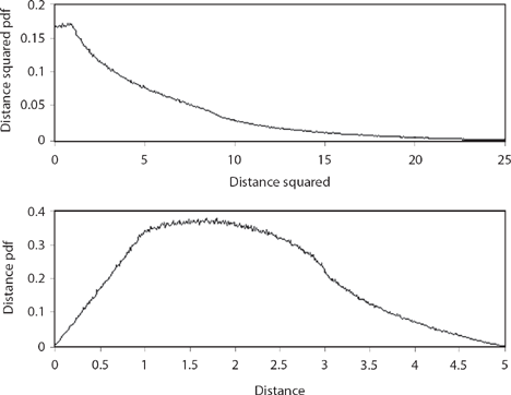
Figure 14.9. Five-step walk.

Notice that (14.9) says and that as r → 0 the pdf levels off and approaches the value of 1/π = 0.3183 for f_R(0), just as the simulation curve in Figure 14.5 suggests (a direct examination of the elements of the pdf vector gives a value of 0.3174 for f_R(0)). All of these calculations suggest the code pearson.m is working correctly.

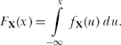
So, what happens for the longer walks that Pearson could not work out analytically?12 Figures 14.8, 14.9, and 14.10 show the distance squared and the distance pdfs for the three-, five-, and six-step random walks, respectively. You can see that while they are distinctly different, at the same time there is a definite pattern to how the pdfs change with an increasing number of steps. The distance pdfs are indeed looking more and more like Rayleigh’s pdf (compare Figure 14.10 with Figure 14.1), while the distance squared pdfs “appear” to be approaching something like an exponential. And that “appearance” leads to the second challenge problem to end this discussion. But first, try your hand at this one.

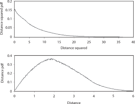
Figure 14.10. Six-step walk.

CP. P14.1:

CP. P14.2:

Notes and References

1. “The Logical Basis of the Sanitary Policy of Mosquito Reduction” (Science, December 1, 1905, pp. 689–699).

2. “The Problem of the Random Walk” (Nature, July 27, 1905, p. 294).

3. Probability can be very practical, too. One of the first topics discussed in any introductory probability course, for example, is combinatorial theory, about which the famous Polish-born American mathematician S. M. Ulam (1909–1984) had this to say in his autobiography Adventures of a Mathematician (Scribner’s 1976, p. 91): “When I became chairman of the mathematics department at the University of Colorado, I noticed that the difficulties of administering N people was not really proportional to N but to N². This became my first “administrative theorem.” With sixty professors there are roughly eighteen hundred pairs of professors. Out of that many pairs it was not surprising that there were some whose members did not like one another.” More precisely, Ulam’s calculation is the binomial coefficient

4. “The Problem of the Random Walk,” p. 318.

5. If you’re wondering why Rayleigh’s probability expression in his letter to Pearson doesn’t have any l-dependency, that’s because Rayleigh has quietly assumed l = 1. Look back at his precise wording, where he speaks of “unit amplitude” oscillations.

6. Saying a random variable X has the pdf fX(x) means that the integral of fX(x) over an interval gives the probability X takes on a value in that interval. If the interval is (—∞, x) then that probability is called the distribution function of X, written as F_X(x) = P(—∞ < X ≤ x) = P(X ≤ x): that is,

In fact, the usual sequence of operations is just the reverse of this, that is, one usually first finds the distribution F_X(x) by other means and then calculates the density as

Rayleigh’s pdf, in particular, appears in countless applications. Here’s just one, of special interest to students of modern intercontinental warfare. If a large number of identical ICBM rockets are independently launched at a distant target, and if one measures the distance between the target and the actual impact point of each missile (the so-called radial miss distance), then the miss distances are the values of a random variable with a Rayleigh pdf. Each type of ICBM has a different Rayleigh pdf, parameterized on what is called the CEP (the initialism for the rather awkward phrase “circular error probability”). The CEP is the radius of the circle centered on the target within which half the missiles will impact (and outside of which the other half will land).

7. “The Problem of the Random Walk,” p. 342.

8. Pearson’s thanks for the n = 3 case were to Geoffrey Thomas Bennett (1868–1943)—the middle initial J. in Pearson’s printed letter was a typo—who was a lecturer in mathematics at Emmanuel College.

9. Much interesting historical discussion on random walks is in the paper by Jacques Dutka, “On the Problem of Random Flights” (Archive for the History of Exact Sciences 32, 1985, pp. 351–375). See also S. Chandrasekhar, “Stochastic Problems in Physics and Astronomy” (Reviews of Modern Physics, January 1943, pp. 1–89).

10. You can find much more on the Monte Carlo approach in my two books, Duelling Idiots (2003) and Digital Dice (2008), both published by Princeton University Press. The two books together, in addition to their historical discussions, contain seventy or so problems, each with a complete, detailed solution in the form of a tested computer code written in MATLAB.

11. A personal note: between my master’s degree and my doctoral degree, I worked for several years (1963–1972) as a digital system logic designer and programmer in the Southern California aerospace business. In those years, writing a computer program in which one casually dimensions a 2 by 2,000,000 matrix would have been considered a fantastic dream for all but those with access to one of the latest super-duper, top-secret computers operated by the National Security Agency. Today it is a routine task for anyone who owns a quite ordinary home computer running the commercial version of MATLAB. In the 1960s, computer memory was made from low-density integrated transistor circuitry, mechanically rotating magnetic drums, or expensive, bulky magnetic cores. To speak of 1,000-gigabyte memory storage units then would have been the signature of madness! Today, however, massive high-speed computer memory is literally cheaper than dirt. This revolution in data storage was recently recognized by the awarding of the 2007 Nobel Prize in Physics for the discoveries that made such massive computer memories commonplace

12. E. Merzbacher, J. M. Feagin, and T-H. Wu, “Superposition of the Radiation from N Independent Sources and the Problem of Random Flights” (American Journal of Physics, October 1977, pp. 964–969). This paper presents computer simulation results that agree with the ones in this discussion (produced by simulating between 100,000 and 200,000 walks, as compared to the 2,000,000 walks used here), as well as the theoretical calculation of the pdf’s of the distance squared for all finite N (the length, in steps, of the walk), following the method developed by the Dutch mathematician J. C. Kluyver (1860–1932) who solved Pearson’s original problem only months after Pearson’s first letter appeared in Nature, not just Rayleigh’s limiting case of N → ∞. In particular, the authors write, “In comparing our results with Pearson’s tables and graphs [in a 1906 paper in which Pearson presented some numerical evaluations of Kluyver’s formal integrals] we generally found satisfactory agreement—remarkable in view of the numerical technology available in 1906—but in a few instances we detected significant differences in detail. For example, while Pearson shows a constant value [in the distance-squared pdf for the five step walk of] 0.169 [over the interval 0 to 1], we noticed a slight rise.” You can see that Figure 14.9 also suggests such a rise over that interval.