Chapter 8: Nematicons in Light Valves

Stefania Residori and Umberto Bortolozzo

INLN, Université de Nice-Sophia Antipolis, CNRS, Valbonne, France

Armando Piccardi, Alessandro Alberucci and Gaetano Assanto

Nonlinear Optics and OptoElectronics Lab, University ROMA TRE and CNISM, Rome, Italy

8.1 Introduction

Solitons are ubiquitous in nature [1] and appear in such different fields as fluid dynamics, plasma physics, acoustics, magnetohydrodynamics, quantum electrodynamics, and Bose–Einstein condensates, just to cite a few. In optics, bright spatial solitons have been identified as nonlinear solutions of the propagation equation when light travels in materials with a dielectric constant increasing with the intensity of light [2]. Optical spatial solitons are self-trapped beams able to create their own dielectric waveguide and propagate in it without diffractive spreading. A wealth of theoretical and experimental work has been devoted to optical solitons, not only for their fundamental interest [3] but also for their potential applications in photonics, waveguiding, and communications [4].

Nowadays, the ability to optically control soliton dynamics, their paths and trajectories, has attracted considerable attention in the perspective of implementing all-optical and parallel architectures in optical interconnects. This chapter discusses optical spatial solitons in liquid crystal (LC) light valves. In these systems, optical spatial solitons arise because of the molecular reorientational nonlinearity of LC, whereas the optical control is provided by a photosensitive layer of the cell.

The first part of this chapter, Section 8.2, is a brief introduction to the reorientational optical nonlinearity of LC and soliton formation in nematics. Section 8.3 provides a general presentation of the liquid crystal light valve (LCLV), with a description of the cell structure and its working principle. Spontaneous pattern formation in the presence of a feedback mirror is also briefly described as an example of transverse configuration. Section 8.4 describes a light valve optimized for the excitation and propagation of spatial solitons in the longitudinal direction of the LC layer, together with the presentation of stable nematicons and of ways of changing their walk-off. Then, Section 8.5 deals with the propagation of solitons in the presence of local and optically induced defects of the molecular orientation. Experiments are discussed together with a theoretical model supporting the observations. Section 8.6 demonstrates how the previously exposed effects can be effectively employed to realize logic gates by optically addressing nematicons. Finally, Section 8.7 concludes and illustrates the perspectives for future work.

8.2 Reorientational Kerr Effect and Soliton Formation in Nematic Liquid Crystals

LC are strongly anisotropic materials composed of elongated organic molecules. Their main feature is that there is a temperature range within which they constitute mesophases, that is, they form phases with properties intermediate between solids and liquids. Different LC phases exist, exhibiting higher or lower degrees of long-range order [5]. The optical properties of LC are very appealing, because of their large birefringence, polarization selectivity, and transparency over the full visible and near-infrared ranges [6].

Nematic LC, the most commonly used especially in liquid crystal displays (LCDs), are characterized by a preferential orientation of the long axes of the molecules. Therefore, in the nematic phase, all molecules are—in average—aligned along a preferential direction, called the nematic director . Because of their anisotropy, LC molecules have different polarizabilities along their long and short axes, with dielectric anisotropy Δ ε = ε _|| − ε _⊥, ε _|| and ε _⊥ being the dielectric constants parallel and orthogonal to , respectively. When an electric field, or a voltage, is applied across the nematic layer, induced dipole moments arise because of such anisotropy and the molecules tend to reorient and become aligned with the direction of the applied field. This process is called Fréedericksz transition and requires the applied field to be high enough to overcome the elastic restoring forces of the LC layer, usually a few volts in common nematic cells [5, 6].

Moreover, a nematic LC layer behaves as a strongly birefringent material, characterized by different refractive indices for light beams polarized parallel or orthogonal to , that is, the extraordinary and ordinary indices, respectively. Typical values of the extraordinary and ordinary indices of a nematic LC (e.g., E7) are n_e = 1.7 and n_o = 1.5, respectively, that is, birefringences as large as Δn = n_e − n_o = 0.2. On applying an electric field, molecular reorientation can lead to a change of the optic axis of the nematic layer as a whole. This allows to control the refractive index and/or birefringence and/or walk-off in the LC layer as a function of the applied voltage. Based on this principle, LCDs exploit changes in transmissivity of a twisted nematic cell placed in between a couple of crossed polarizers [7].

8.2.1 Optically Induced Reorientational Nonlinearity

It is also possible to drive the (re)orientation of the LC molecules by using directly the electric field of a light beam impinging on the nematic layer. When the polarization of the incoming beam is such that the projection of the electric field on the nematic director is zero (ordinary wave) we usually refer to it as the optical Fréedericksz transition (OFT) [8]. In this case, there is a threshold for molecular reorientation to occur and, indeed, OFT requires intensities as high as a few hundred kiloWatts per square centimeter. At powers below the Fréedericksz threshold, molecular reorientation occurs only if the beam polarization has a nonzero projection on the nematic director, that is, reorientation can be triggered only by an extraordinary wave component.

When, due to the action of a light beam, molecules reorient, they change direction toward the polarization of the input field if the high frequency dielectric anisotropy, , is positive [6]. Therefore, optically induced reorientation leads to a change of the refractive index from its lower to higher values, that is, from ordinary to extraordinary index in OFT [9]. The amount of reorientation, therefore, of refractive index change is proportional to the input beam intensity, which provides a self-focusing Kerr-like effect [10]. Focusing Kerr nonlinearities can, in general, be exploited to compensate beam spreading due to diffraction, allowing to generate bright spatial solitons [2–4]. As we see in the following sections, the reorientational effect in nematic LC has been proved to be an efficient mechanism to create spatial optical solitons.

8.2.2 Spatial Solitons in Nematic Liquid Crystals

Optical spatial solitons result from the balance of diffraction and self-focusing in nonlinear media; their transverse index profile is able to confine the soliton as well as other signals [3, 4]. In nematic LC, solitons arise from the balance of diffraction with the self-focusing molecular reorientation under the action of an extraordinarily polarized field.

Pioneering experiments on optical solitons in LC were reported for a laser beam propagating in a capillary tube filled with nematics [11]. It was shown that a beam propagating inside a nematic layer undergoes a strong self-focusing effect followed by filamentation, or soliton formation, when the light intensity increases. Since then, stable and controllable spatial solitons in nematics, also called nematicons, have been obtained in planar cell geometries [12]. It was shown that nematicons can be controlled by changing their route by modifying their walk-off and/or the perceived refractive index, thanks to the application of an external low-frequency electric field (Chapter 5). Nematicons have, thus, been proved to be excellent candidates for signal readdressing and processing in reconfigurable circuits [13, 14].

Modulational instability regimes were also studied in similar setups [15, 16], showing the spontaneous filamentation of initially uniform extended beams on propagation in a nematic layer. Recently, a new mechanism for spontaneous soliton formation has been devised and experimentally proved, which is based on the establishment of optical wave turbulence, characterized by low nonlinearity and spontaneous soliton formation at very long distances inside a nematic planar cell after the propagation of an extended (and with initial phase noise) beam [17].

The theoretical framework for soliton formation and beam filamentation in nematics is very general and includes two coupled differential equations, one describing the noninstantaneous and nonlocal (diffusive) response of the LC and the other accounting for the beam propagation, namely (see Chapter 1)

8.1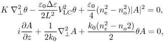

where θ is the molecular orientation angle in the LC layer, in the linear approximation and for θ around θ₀ = π/4; K is the LC elastic constant, taken equal for splay, twist, and bend (one constant approximation); Δ ε is the LC dielectric anisotropy; A is the amplitude of the optical field; k₀ is the optical wave number; and ε ₀ is the vacuum permittivity.

In the past decade, a high degree of control, such as routing and steering of nematicons, has been achieved by varying the voltage applied across the nematic slab (Chapter 5) [12–14]. However, an all-optical control of spatial solitons is highly desirable in order to optimize the routing/steering process, to achieve high levels of parallelism, to realize flexible multiplexing configurations, and to allow interconnects to be reconfigured in real-time. In view of implementing such all-optical control protocols, preliminary attempts were carried out with intense external beams, also using azo-dye-doped LC and surface effects [18–20]. More recently, a finely controllable setup has been realized by using an LCLV in place of a standard planar cell [21]. Stable nematicons were created in the light valve and the photo-controlled transduction of light into effective voltage across the LC layer, due to the valve operation, allowed for a flexible and all-optical control of the nematicon dynamics.

8.3 Liquid Crystal Light Valves

LCLV are optically addressable spatial light modulators, able to impose a phase modulation on the wave front of a readout beam, whereas the control/input signal is provided by another optical beam [22]. The general structure of an LCLV comprises two components, the photoreceptor and the electro-optic material, sometimes separated by a dielectric mirror [23]. Historically, the photoreceptor was a photoconductor, such as selenium or cadmium sulfide [24], amorphous silicon [25] or GaAs [26]. Therefore, in general, LCLV are hybrid structures, combining organic layers—typically made of nematic LC—with solid-state photosensitive substrates. The input beam activates the photoreceptor, which produces a corresponding charge field on the electro-optic material. The readout light is modulated in its double pass through the electro-optic element in a retroreflective scheme.

More recently, photorefractive LCLV have been realized by combining a nematic LC layer with a thin monocrystalline Bi₁₂SiO₂₀ (BSO) crystal [27]. The BSO, well known for its photorefractive properties [28], was chosen for its large photoconductivity and transparency in the visible range together with the possibility of having large monocrystalline samples with good optical quality and uniform dark resistance. The maximum photoconductivity of the BSO is in the blue-green region of the spectrum. The photorefractive LCLV is a novel type of spatial light modulator that works in transmissive configurations, where input and readout beams may in general coincide. We see, in the following discussion, how this type of LCLV can be optimized for the generation and all-optical control of nematicons.

8.3.1 Cell Structure and Working Principle

A typical BSO-made LCLV is sketched in Figure 8.1. A thin layer of nematic LC is sandwiched between a glass plate and a wall made of the photorefractive BSO crystal, cut in the shape of a thin plate (1 mm thickness, 20 × 30 mm² lateral size). Before assembling the cell, the inner surfaces of both the BSO and the glass plate are coated with polyvinyl alcohol polymer and mechanically rubbed to obtain the planar alignment of the LC (nematic director parallel to the confining walls). After this treatment, the gap between the two walls, of typical thickness L = 14μm, is filled with the LC. Transparent electrodes, made of indium tin oxide (ITO) are deposited on the outer surface of the BSO and the inner surface of the glass plate: they allow applying an external bias V₀ across the cell.

When an electric field is applied across the nematic layer, all the molecules tend to reorient in such a way that they become aligned with the direction of the applied field. This implies a change in the optic axis of the LC layer; hence, an incoming light field experiences a large refractive index change. Typically, the voltage applied is AC, with a root mean square rms value from 2 V to 20 V and a frequency from 50 Hz to 20 kHz. When a light beam impinges on the LCLV, because of the photoconductivity of the BSO, photogeneration of charges occurs at its surface; hence, the effective voltage across the LC layer increases locally, according to the illumination. As a consequence, the LC molecules reorient and, due to their birefringence, the light beam acquires a phase shift φ at the exit of the valve, which is a function of the applied voltage and of the beam intensity itself.

A typical response function of the LCLV is shown in Figure 8.1b, where the phase shift φ acquired by the light beam passing through the valve is plotted against the input beam intensity I. The response is linear up to intensities of the order of 10 mW/cm². Then, it saturates to a value that corresponds to the maximum birefringence, Δn ≈ 0.2, when all the LC molecules are aligned along the direction of the applied field. In between, that is, from the initial planar alignment to the final orthogonal alignment, the average orientation angle of the LC molecules varies from 0 to π/2, leading to a phase shift φ that, in the linear part of the LCLV response, changes from 0 to several π. In this range of parameters, the LCLV behaves as a Kerr-like medium, providing an effective change of the refractive index proportional to the input light intensity. Correspondingly, the LCLV nonlinear coefficient is as large as n₂ − 6 cm²/ W, the minus sign accounting for the defocusing character of the nonlinearity (the refractive index changes from n_e to n_o when increasing the voltage or the light intensity) [29].

The response time of the LCLV is dictated by the time τ_LC required for the collective motion of the LC molecules to establish over the whole thickness of the nematic layer. This is given by [5]

8.2

where γ is the LC rotational viscosity and K is the LC elastic constant (taken equal for splay, twist, and bend deformations). For L = 14μm and typical values of the LC constants, τ_LC is of the order of 100 ms. Note that, owing to the slow relaxation time, the LC molecules cannot follow the oscillation of the applied AC field. Instead, they perform a static reorientation, in which they reach an equilibrium position fixed by the rms value of the voltage. Because of the complex impedances of the different layers comprising the LCLV, there is an optimal frequency range within which the contrast of the voltage transferred to the LC with and without illumination is maximum [27, 29, 30].

Finally, the nonlinear mechanism in the LCLV is different from optically induced reorientation, even though both deal with orientation of the LC molecules. Indeed, whereas in the LCLV nonlinearity the molecules are driven by the low-frequency external bias and light intervenes through the photoconductive transducer, in the second case molecules are directly oriented by the electric field of the incoming light beam. This second mechanism requires much higher intensity for obtaining an equivalent distortion of the nematic layer. In the LCLV, the two effects combine for the control of spatial soliton propagation: nematicons can be excited via optically induced reorientation, whereas the LCLV nonlinearity allows local and dynamical addressing of the refractive index.

8.3.2 Optical Addressing in Transverse Configurations

Transverse configurations have been used to address the LCLV in various nonlinear optical experiments. In particular, spontaneous pattern formation in the presence of an optical feedback and by using a retroreflective LCLV have been largely studied in the past, showing different types of spatial structuring of the optical wave front and various spatiotemporal dynamical regimes [26, 31–33]. For the same type of retroreflective LCLV, the control of optical localized structures [34] and the control of front propagation dynamics [35] have been efficiently implemented by illuminating the photoconductive side of the valve with suitable spatially modulated optical potentials.

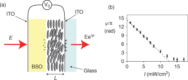
More recently, the BSO-made transmissive LCLV has allowed more simplified schemes for optical feedback experiments [36]. Figure 8.2a shows the typical setup for spontaneous pattern formation under transverse optical feedback. In the linear part of its response, the LCLV can be assimilated to a Kerr medium, providing a phase change proportional to the input intensity (Fig. 8.1b). In the presence of a feedback mirror placed at a distance d/2 with respect to the LCLV, any initial amplitude perturbation is converted into phase modulation by the nonlinear response of the LCLV, whereas the free propagation from the valve to the mirror reconverts phase into amplitude modulation [31]. If the light intensity is increased above a certain threshold, an instability takes place and makes the initially uniform wave front become spatially structured, as shown in Figure 8.2b. The spatial period of the structure, , is a geometric mean of the total free propagation length d and of the light wavelength λ. For a laser wavelength in the visible, it is typically of the order of a few hundred micrometers for d of the order of a few centimeters and can be easily changed by varying the distance between the valve and the mirror.

The transmissive configuration of the photorefractive light valve also offers the possibility of performing wave mixing experiments [29, 37]. The beam coupling takes place over a large working area, and extra optical/electric control can be achieved by addressing the photoconductive layer. Two-wave mixing experiments have led to signal beam amplification [38] and the realization of nonlinear optical cavities [39, 40] as well as to slow-light experiments [41].

Finally, it is worth mentioning the possibility of addressing the BSO with arbitrary distributions or optical potentials. For instance, controlled distributions of disorder have been used to illuminate the photoconductive side of the valve, inducing corresponding distributions of defects in the molecular orientation; the latter has provided experimental evidence of speckle instability under the simultaneous presence of disorder and nonlinearity [42].

8.4 Spatial Solitons in Light Valves

For the propagation of stable spatial solitons we have prepared specific BSO-made light valves aimed at favoring the self-guided propagation in a longitudinal dimension of the LC layer [21]. To this end, we have employed large sample thicknesses and oblique planar anchoring at the surfaces. The first condition facilitates the in-coupling of the beam in the LC layer, whereas the second one is used to favor the optically induced reorientation.

8.4.1 Stable Nematicons: Self-Guided Propagation in the Longitudinal Direction

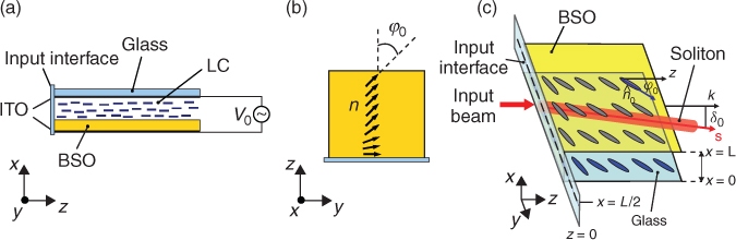
A schematic drawing of the soliton-optimized LCLV is shown in Figure 8.3. It consists of a glass slide and a photoconductor slab of BSO, both coated with a layer of ITO for the application of an external voltage bias and held parallel to one another by 50 μm Mylar spacers to obtain the necessary thickness. An additional glass slide is sealed on one side of the LCLV (see Figure 8.3a) and provides the interface for launching the input beam, thus preventing depolarization and meniscus effects at the entrance of the LC layer. All the internal surfaces are coated with a polyvinyl alcohol polymer and mechanically rubbed to provide molecular anchoring and alignment in the nematic phase. As shown in Figure 8.3b, the rubbing is parallel to y on the input facet to optimize the coupling of the extraordinary wave in the bulk NLC; in the bulk φ₀ is the angle of the initial with , being as well. Once assembled, the LCLV is filled with the nematic LC E48, with n_|| = 1.7536 and at the employed wavelength. Figure 8.3c sketches the typical experimental configuration for soliton excitation. Typically it is φ₀ = π/4, in order to maximize the optical nonlinearity, and δ₀ is the soliton walk-off.

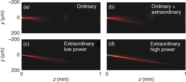
A TEM₀₀ mode from a He–Ne laser, wavelength 632.8 nm, is focused onto the cell entrance at x = L/2 with a waist of about 6 μm and wave vector . We use an optical microscope and a camera to image the beam evolution in the y–z plane, collecting the photons scattered by the LC out of the plane of propagation. In order to characterize the LCLV as a suitable environment for nematicon propagation, the applied voltage is first set to V₀ = 0 V. Optically induced reorientation occurs for the extraordinary beam when the intensity is sufficiently high. Sample results are shown in Figure 8.4. When the beam is polarized parallel to x (ordinary wave), we observe diffraction independent of excitation, as shown in Figure 8.4a. Conversely, when the beam is polarized parallel to y (extraordinary wave), self-focusing compensates diffraction and gives rise to spatial solitons for powers greater than or equal to 1.5 mW, as can be seen in Figure 8.4d. In Figure 8.4b a mixed polarization state (electric field linearly polarized at π/4 with respect to both x and y) and P = 2.5 mW yields a diffracting beam for the ordinary component and a nematicon for the extraordinary component. In Figure 8.4c, the extraordinary polarized beam diffracts at low power, P < 1 mW.

Owing to the large birefringence of E48, with Δn ∼ 0.23, solitons propagate with a Poynting vector at a large walk-off angle δ₀ ∼ 7^° with respect to their wave vector . The Poynting vectors corresponding to ordinary and extraordinary beam excitations are visible in Figure 8.4b. Once excited, nematicons propagate as self-confined beams over distances exceeding 15 Rayleigh lengths, that is, as long as their power remains high enough in spite of the propagation (scattering) losses.

8.4.2 Tuning the Soliton Walk-Off

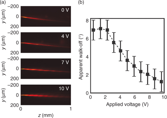
The soliton walk-off in the y–z plane can be changed by the application of a voltage V₀ across the LC thickness, as previously done in standard LC cells (Chapter 5) [12]. In the LCLV, we apply a low-frequency voltage of variable (rms) amplitude across the cell and record the corresponding soliton paths [21]. The results are shown in Figure 8.5. Figure 8.5a shows the nematicon propagation for various applied voltages. Correspondingly, Figure 8.5b plots the measured soliton walk-off. For voltages above 2 V (corresponding to the Freedericksz threshold for reorientation), the apparent walk-off (i.e., the observable angle between and ) reduces, approaching 0° for a bias V₀ = 6 V such that the director becomes nearly parallel to x and no further molecular reorientation takes place. Thereby, when δ approaches zero the beam loses self-confinement because the nonlinearity fades away, as apparent from the bottom photograph in Figure 8.5a. We stress how the curve in Figure 8.5b follows the qualitative behavior of standard LC samples, but differs for the voltage scale, owing to the equivalent resistance of the BSO layer [12].

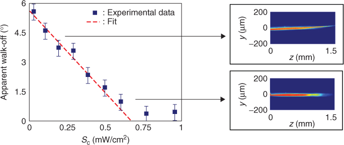
Other than via the applied voltage, the nematicon walk-off in the LCLV can be optically controlled by uniformly illuminating the BSO, thanks to its photoconductive properties. For a fixed bias and under uniform external illumination with an expanded laser beam, the LC layer where a nematicon propagates can be tuned in orientation. To illuminate the LCLV, we use a solid-state laser operating at 532 nm, well within the spectral range where the BSO has maximum photoconductivity. Then, we launch a 2 mW nematicon at 632.8 nm as described earlier and keep the bias fixed at V₀ = 3.5 V and frequency f = 80 Hz while varying the external beam intensity. Figure 8.6 shows the measured change in propagation angle (apparent walk-off) versus the external control intensity I_ext. We can see that the walk-off is efficiently controlled by the external light; hence, the soliton is angularly steered, in analogy to what is observed in Figure 8.5 but now by way of an all-optical control.

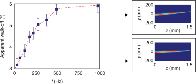
Another important feature of the LCLV is the response time introduced by both LC and photoconductive layers when the external electric field is applied: whereas the former, dictated by the time of LC molecules to be reoriented (typically in 100 ms, Chapter 13), does not allow a frequency below 10 Hz, the latter imposes an upper bound, determined by the BSO–LC equivalent electrical impedance. This cutoff frequency can be observed in Figure 8.7, showing the apparent walk-off under voltage bias and illumination versus frequency: clearly, no change in nematicon trajectory occurs above 500 Hz.

To establish a direct comparison between electrical and optical control of the walk-off, we resort to a simple model describing the photoconductor response in the linear approximation [33]. In this case, the effective voltage applied to the LC layer can be expressed as

8.3

where Γ accounts for the impedances of the dielectric layers and α is a phenomenological parameter describing the linear response of the photoconductor in the LCLV. The values Γ = 0.6 and α = 3 · 10³ Vcm²/W apply to our valve; hence, as the external intensity I_ext varies from 0 to 1 mW/cm² in a fixed bias LCLV, the latter operates as if the applied voltage V₀ increases from 0 to 5 V (i.e., increases in V_LC from 0 to 3V). For a fixed bias V₀ = 3.5 V and increasing the illumination as earlier, conversely, the walk-off varies linearly with an equivalent voltage dynamics from V₀ = 3.5 to V₀ = 8.5 V (i.e., V_LC from 2.1 to 5.1 V). Linearity breaks down above I_ext = 0.7 mW/cm², when saturation of the nematic response (director parallel to the quasistatic electric field) comes into play.

8.5 Soliton Propagation in 3D Anisotropic Media: Model and Experiment

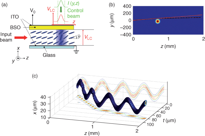
The photoconductive transduction of intensity into applied voltage across the LC layer allows for selectively addressing local areas of the LC underneath the BSO. Then, local control of the soliton trajectory can be implemented by using finite size external beams rather than uniform illumination of the BSO [43, 44]. To this purpose, a small spot laser beam at 532 nm can be employed to induce lenslike director/index perturbations along the path of nematicons, as sketched in Figure 8.8a. The solitons propagating in the vicinity of a light-induced defect in the molecular order can sense a change in refractive index and a local variation of walk-off, bending their trajectories along paths depending on the distance from the perturbation, its size, and its shape (see Figure 8.8b–c).

The propagation of nematicons near externally induced “defects” along a local longitudinal coordinate z can be modeled—in the most general case—by a set of coupled partial differential equations, including the Poisson equation governing the electrostatic potential, the reorientational equations governing the director distribution (determined by two angles that fix the local orientation of the director), and finally, the Maxwell equations ruling light evolution. The solution of this complete model is quite heavy, but some drastic simplifications can be applied in order to enlighten the fundamental concepts and, at the same time, to save computational power. In order to determine the molecular director distribution in the presence of a voltage and external control beam, we have to compute the two angles θ and φ that the director makes, respectively, with z in the x–z plane and with z in the y–z plane throughout the bulk LC (Fig. 8.9) when a soliton propagates in the LCLV [45]. By considering all the various contributions, we have θ = θ_Vc + θ_NL and φ = φ_Vc + φ_NL, where θ_Vc ≡ θ_V + θ_c and φ_Vc ≡ φ_V + φ_c are the background values due to the bias, θ_V, φ_V, and to the control beam, θ_c, φ_c, respectively, and θ_NL, φ_NL are the nonlinear (reorientational) perturbations induced by the spatial soliton. The soliton-induced perturbations at typical experimental powers (<3 mW) are negligible with respect to θ_Vc and φ_Vc; hence, we can safely take θθ_Vc and φφ_Vc, that is, the soliton does not appreciably modify the defect when passing nearby. Moreover, by assuming an infinitely extended cell in the y–z plane, we can also take θ_V = θ_V(x) and φ_V = φ₀ throughout the LC volume, φ₀ fixed by anchoring. The low-frequency electric field effectively acting on the LC is increased by the control-beam-induced charges via the associated decrease in BSO resistivity, with behavior roughly dictated by Equation 8.3. We do not account for variations of the intensity I_ext along x, as the control beam can be considered collimated inside the BSO layer. We also assume that the low-frequency electric field components lying in the y–z plane are negligible with respect to the x-component; hence, only θ_Vc changes under the action of V_LC. This is physically plausible because owing to the geometry and the dielectric constant of BSO larger than the LC ( ε _BSO = 56, ε _|| = 19.5) [28], the field lines in yz concentrate in the BSO slab. In the single elastic constant approximation, the reorientation equation in 3D takes the form

8.4

where γ = ε ₀Δ ε /(2K). As said earlier, at standard intensities the torque due to direct coupling between the control beam and the LC molecules can be neglected. We can, thus, solve Equation 8.4 with the proper boundary conditions to determine the director profile around the defect [46].

Once the optic axis distribution in the LC volume for a given control spot or defect is known, we only have to determine light propagation in such index landscape. In particular, we are interested in computing the soliton trajectory for adiabatic changes in the dielectric tensor and in the limit of high nonlocality, consistent with the experimental conditions. Under them, the evolution of the beam envelope A can be found via the scalar equation

8.5

where Ψ and ψ are the local angle between wave vector and director in the absence of a soliton and its nonlinear variation, respectively, and D_y is the diffraction coefficient along y. The reference system x_ly_lz_l is a moving frame rotating with the beam such that z_l and y_l are always parallel to the local wave vector and electric extraordinary displacement vector, respectively. Equation 8.5 holds valid in the paraxial approximation and for a director distribution slowly varying with respect to the intensity width (Chapter 5). We are now able to compute the soliton trajectory: explicitly, after defining the position of the soliton center of mass as

8.6

and applying the Ehrenfest theorem to Equation 8.5, we find

8.7

with the force , normal to the local wave vector, given by

8.8

The superscript “(b)” indicates the extraordinary refractive index computed at the beam peak. The first two terms on the right-hand side of Equation 8.8 are due to index gradients as in isotropic media; the third term is directed along y_l and stems from anisotropy: it accounts for longitudinal changes in walk-off.

Equation 8.7 predicts a soliton path independent of waist. Moreover, in our experimental conditions the transverse force always attracts the soliton toward the axis of the defect induced by the control beam, as the extraordinary refractive index is larger where V_LC is higher. In the absence of external illumination, the soliton evolves with sinusoidal oscillations in xz because of the joint action of walk-off and of the index well created by the bias. In the plane y–z, the soliton appears to propagate straight, with slope tan(δ_yz), tan(δ_yz) being the apparent walk-off [12].

An example of measured and calculated nematicon bending in the light valve near a light-induced lenslike perturbation is shown in Figure 8.8b, with an excellent agreement between model and experiment. Figure 8.8c displays the three-dimensional trajectory of a nematicon under the influence of the transverse electric potential (bias) and the defect. Owing to both walk-off out of the propagation plane y–z and refractive index perturbation, the soliton propagates oscillating up and down in the valve while bending its trajectory; hence, it moves in a complex 3D path distorted by both bias and illumination [43].

8.5.1 Optical Control of Nematicon Trajectories

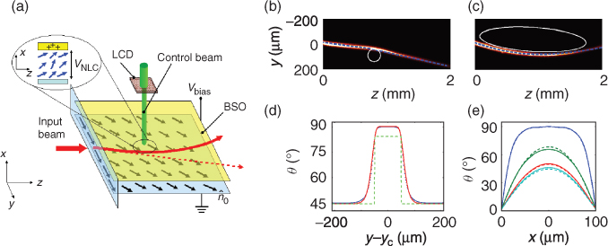
Rather than a small beam, arbitrary shape and size perturbations can be applied by means of an external spatial light modulator (or LCD). To realize a 3D configuration of soliton control, the profile of the control spot(s) is adjusted by using a programmable LCD as shown in Figure 8.9a. Examples of curved soliton paths due to circular and elliptically shaped spots are shown in Figure 8.9b–c for V₀ = 5 V, I_ext = 100 μ W/cm², and 2 mW solitons launched with wave vector and Poynting vector at walk-off δ₀ = 7^° with respect to the axis z. Noteworthy, flat-top beams are employed in order to maximize the light-induced index gradient for a fixed difference between maximum and minimum indices.

The computed trajectories are in excellent agreement with the experimental data, as visible in Figure 8.9b–c, dashed lines. For a control spot with small curvature (Fig. 8.9b), the soliton senses a pointlike perturbation and is deflected toward its center. For lesser curvature (Fig. 8.9c) the soliton is able to follow the profile edge, as the effective force due to the index gradient is weaker. Finally, Figure 8.9d–e shows the director distribution θ_Vc along y (x) when a circular control beam shines the photoconductor, with voltage V₀ and control intensity I_ext so as to saturate the director reorientation and maximize the gradient in dielectric tensor. The flat-top shape of the control beam (dashed lines) is smoothed in the LC because of the nonlocal response, with length of the transition zone fixed by the width of the reorientational response (Chapter 11).

8.6 Soliton Gating and Switching by External Beams

The optical potential previously superposed on the nematicon can be dynamically modified by acting on the programmable LCD in order to implement the desired soliton operations [47]. By using the model introduced earlier and the LCD spatial modulator, we can design and demonstrate a number of low power optically driven routers and logic gates, with logic input represented by the control spots and signal carried by solitons.

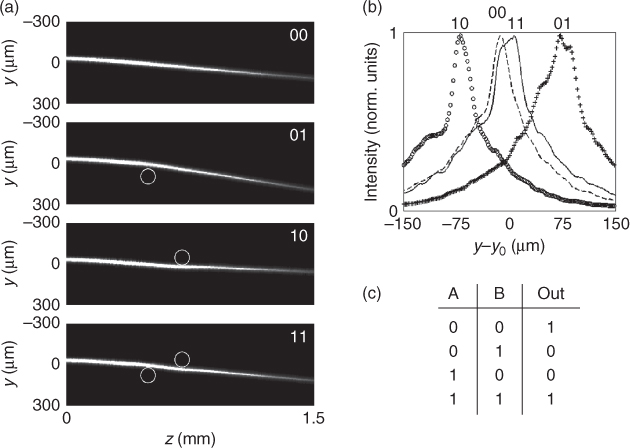
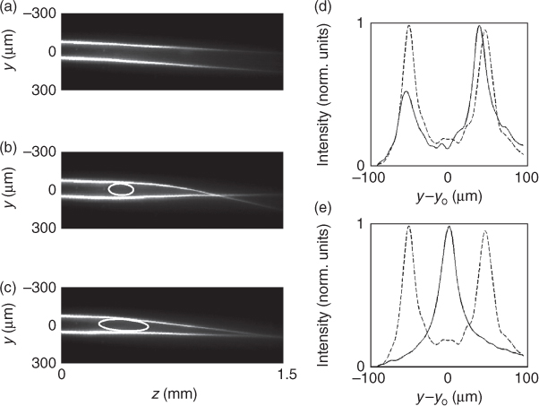
Figure 8.10 shows an experimental implementation of an XNOR gate, with the soliton output y-position equal to the unperturbed one y₀ (i.e., in the absence of control beams) corresponding to a high (true) logic state, equivalent to a low (false) state if the soliton is located elsewhere. As demonstrated by the evolution in yz (Fig. 8.10a) and by the acquired transverse profiles (Fig. 8.10b), the evolution without perturbation (00) and with both control inputs (11) leads the soliton to the same output y₀: this is achieved by a proper choice in the positions of the two control beams (power and shape are equal) such that the deflection from the rightmost defect exactly compensates the deviation due to the leftmost control beam.

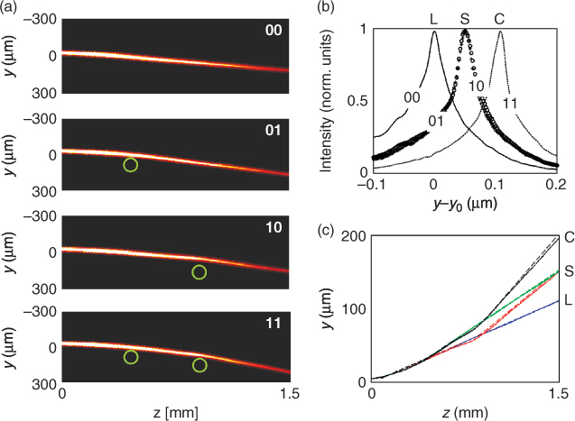
Having experimentally demonstrated all-optical logic gating in LCLV, our next step is a half adder (HA), that is, the building block of any digital processor. Figure 8.11 demonstrates the realization of a binary all-optical HA in LCLV. In fact, when only one control beam is turned on, the soliton output position remains the same no matter which input is on; the output position is labeled S (Fig. 8.11b,c) and gives the Sum bit (in this case a high logic state). Consistent with the previous definition, S is dark (low logic state) when the two control beams are both turned on or off. The output position when both control beams are on can be taken as the carry bit (labeled C in Figure 8.11b–c): for every other pair of logic inputs, C remains low. It is noteworthy that such configuration is quite versatile: in fact, different logic gates can be realized by taking each output position as the unique output state. The geometry in Figure 8.11 acts as an AND, XOR, and NOR when the output position corresponds to C, S, and L, respectively. Finally, Figure 8.11c compares acquired and calculated soliton trajectories, with good agreement.

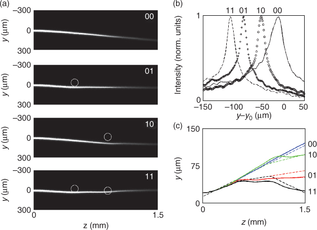
Having demonstrated the all-optical logic gates in LCLV, we are interested in realizing other fundamental devices for signal processing: routers. To realize a digital two-bit router we employ two circular control beams of equal size and shape, and associate their presence or absence with true (high) or false (low) input bits, respectively. Every combination (out of 2² = 4) of Boolean inputs is able to reroute a spatial soliton (and the signal traveling within it) to a different output at a given z. The operation of this 1 × 4 spatial demultiplexer is illustrated in Figure 8.12a, the transverse profiles shown in Figure 8.12b yield an effective cross-talk of about −5 dB, while the solid (dashed) lines in Figure 8.12c are the acquired (calculated) trajectories.

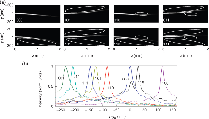
Taking advantage of soliton deflection versus shape of control spots, we can use elliptical spots to increase the deviations and realize a three-bits router, as illustrated in Figure 8.13. By choosing a suitable assortment of elliptical spots at given positions, the spatial soliton can be steered over a wider transverse interval of 400 μm, thus implementing a 1 × 8 demultiplexer controlled by combinations (out of 2³ = 8) of three binary inputs. In this case, the measured cross-talk of about −2.5 dB is due to the smaller distance between different control spots (bits) with respect to the 1 × 4 demultiplexer mentioned earlier.

Besides digital functions, with the LCLV one can build simple analog signal processors: we use the control spots to modulate nematicon–nematicon interaction (Chapter 1) in order to realize X and Y junctions. As shown in Figure 8.14a–d, two nematicons (each of them of power of P = 2 mW to ensure self-confinement) are launched with parallel wave vectors in the plane y–z, but displaced along y of d ≈ 100 μm. The input separation is larger than the cell thickness, that is, the nonlocality range: hence, the index profiles of the two solitons do not overlap in the absence of control spots, preventing soliton–soliton interactions [48]. Conversely, when a “defect” is turned on between the two solitons, the beams are attracted to the defect and to one another, thereby interact. By varying curvature and position of the defect, the two beams can undergo either strong attraction—eventually crossing and forming an X junction (Fig. 8.14b,d)—, or weak interaction—merging at the output (Fig. 8.14c,e) and forming a Y junction [44, 47].

8.7 Conclusions and Perspectives

In conclusion, we have shown that 3D control of nematicon trajectories can be realized through external beam addressing/multiplexing in LCLV. Nematicons have been shown to be robust and predictable solutions of the propagation in specifically designed light valves, with theoretical models confirming and supporting the observations. Gating and switching of solitons has been implemented by using arbitrary shape, position, and size of the control beams by means of a commercially available spatial light modulator.

New scenarios are foreseen in LCLV via the interplay of transverse patterns and propagating solitons [32].

Finally, we like to stress the unique wealth of possibilities offered by LCLV for implementing all-optical controlled schemes of light propagation and localization.

Acknowledgments

S.R. and U.B. acknowledge the financial support of the ANR international program, Project ANR-2010-INTB-402-02, “COLORS”. A.A. thanks Regione Lazio for financial support.

References

1. A. C. Newell. Solitons in Mathematics and Physics. SIAM, Philadelphia, PA, 1985.

2. R. Y. Chiao, E. Garmire, and C. H. Townes. Self-trapping of optical beams. Phys. Rev. Lett., 13:479–482, 1964.

3. Y. S. Kivshar and G. P. Agrawal. Optical Solitons. Academic Press, San Diego, CA, 2003.

4. G. I. Stegeman and M. Segev. Optical spatial solitons and their interactions: universality and diversity. Science, 286:1518–1523, 1999.

5. P. G. De Gennes and J. Prost. The Physics of Liquid Crystals, 2nd edn. Oxford Science Publications/Clarendon Press, Oxford, 1993.

6. I. C. Khoo. Liquid Crystals: Physical Properties and Nonlinear Optical Phenomena, 2nd edn. Wiley Interscience, New York, 2007.

7. P. Yeh and C. Gu. Optics of Liquid Crystal Displays. Wiley, New York, 1999.

8. N. V. Tabiryan, A. V. Sukhov, and B. Zeldovich. Orientational optical nonlinearity of liquid crystals. Mol. Cryst. Liq. Cryst., 136:1–139, 1986.

9. I. C. Khoo. Nonlinear optics of liquid crystalline materials. Phys. Rep., 47:221–267, 2009.

10. J. V. Moloney and A. C. Newell. Nonlinear Optics. Addison-Wesley, Redwood City, CA, 1991.

11. E. Braun, L. P. Faucheux, and A. Libchaber. Strong self-focusing in nematic liquid crystals. Phys. Rev. A, 48:611–622, 1993.

12. M. Peccianti, C. Conti, G. Assanto, A. De Luca, and C. Umeton. Routing of anisotropic spatial solitons and modulational instability in nematic liquid crystals. Nature, 432:733–737, 2004.

13. M. Peccianti and G. Assanto. Nematic liquid crystals: a suitable medium for self-confinement of coherent and incoherent light. Phys. Rev. E, 65:035603, 2002.

14. M. Peccianti, A. Dyadyusha, M. Kaczmarek, and G. Assanto. Tunable refraction and reflection of self-confined light beams. Nat. Phys., 2:737–742, 2006.

15. M. Peccianti, C. Conti, and G. Assanto. Optical modulational instability in a nonlocal medium. Phys. Rev. E, 68:025602, 2003.

16. C. Conti, M. Peccianti, and G. Assanto. Complex dynamics and configurational entropy of spatial optical solitons in nonlocal media. Opt. Lett., 31:2030–2032, 2006.

17. U. Bortolozzo, J. Laurie, S. Nazarenko, and S. Residori. Optical wave turbulence and the condensation of light. J. Opt. Soc. Am. B, 26:2280–2284, 2009.

18. A. Pasquazi, A. Alberucci, M. Peccianti, and G. Assanto. Signal processing by opto-optical interactions between self-localized and free propagating beams in liquid crystals. Appl. Phys. Lett., 87:261104, 2005.

19. S. V. Serak, N. V. Tabiryan, M. Peccianti, and G. Assanto. Spatial soliton all-optical logic gates. IEEE Photon. Technol. Lett., 18:1287–1289, 2006.

20. A. Piccardi, G. Assanto, L. Lucchetti, and F. Simoni. All-optical steering of soliton waveguides in dye-doped liquid crystals. Appl. Phys. Lett., 93:171104, 2008.

21. A. Piccardi, U. Bortolozzo, S. Residori, and G. Assanto. Spatial solitons in liquid-crystal light valves. Opt. Lett., 34:737–739, 2009.

22. U. Efron and G. Liverscu. Spatial Light Modulator Technology: Materials, Devices and Applications. Dekker, New York, 1995.

23. D. Armitage, J. I. Thackara, and W. D. Eades. Photoaddressed liquid crystal spatial light modulators. Appl. Opt., 28:4763–4771, 1989.

24. J. Grinberg, A. Jacobson, W. P. Bleha, and L. Miller. A new real-time non-coherent to coherent light image converter - The hybrid field effect liquid crystal light valve. Opt. Eng., 14:217–225, 1975.

25. P. R. Ashley and J. H. Davis. Amorphous silicon photoconductor in a liquid crystal spatial light modulator. Appl. Opt., 26:241–246, 1978.

26. S. A. Akhmanov, M. A. Vorontsov, and Y. Y. Ivanov. Large-scale transverse nonlinear interactions in laser beams; new types of nonlinear waves; onset of optical turbulence. JETP Lett., 47:707–711, 1988.

27. P. Aubourg, J. P. Huignard, M. Hareng, and R. A. Mullen. Liquid crystal light valve using bulk monocrystalline Bi₁₂SiO₂₀ as the photoconductive material. Appl. Opt., 21:3706–3712, 1982.

28. P. Günter and J. P. Huignard. Photorefractive Materials and their Applications 1. Springer, Berlin, 2006.

29. U. Bortolozzo, S. Residori, and J. P. Huignard. Beam coupling in photorefractive liquid crystal light valves. J. Phys. D: Appl. Phys., 41:24007, 2008.

30. A. Brignon, I. Bongrand, B. Loiseaux, and J. P. Huignard. Signal-beam amplification by two-wave mixing in a liquid-crystal light valve. Opt. Lett., 22:1855–1857, 1997.

31. S. Residori. Patterns, fronts and structures in a liquid-crystal-light-valve with optical feedback. Phys. Rep., 416:201–274, 2005.

32. O. Descalzi, M. G. Clerc, S. Residori, and G. Assanto Eds. Localized States in Physics: Solitons and Patterns. Springer-Verlag, Berlin, Heidelberg, 2011.

33. M. G. Clerc, A. Petrossian, and S. Residori. Bouncing localized structures in a liquid-crystal light-valve experiment. Phys. Rev. E, 71:015205, 2005.

34. U. Bortolozzo and S. Residori. Storage of localized structure matrices in nematic liquid crystals. Phys. Rev. Lett., 96:037801, 2006.

35. F. Haudin, R. G. Elías, R. G. Rojas, U. Bortolozzo, M. G. Clerc, and S. Residori. Driven front propagation in 1D spatially periodic media. Phys. Rev. Lett., 103:128003, 2009.

36. U. Bortolozzo, S. Residori, A. Petrosyan, and J. P. Huignard. Pattern formation and direct measurement of the spatial resolution in a photorefractive liquid crystal light valve. Opt. Commun., 263:317–321, 2006.

37. U. Bortolozzo, S. Residori, and J. P. Huignard. Slow-light through nonlinear wave-mixing in liquid crystal light-valves. C. R. Physique, 10:938–948, 2009.

38. U. Bortolozzo, S. Residori, and J. P. Huignard. Enhancement of the two-wave-mixing gain in a stack of thin nonlinear media by use of the Talbot effect. Opt. Lett., 31:2166–2168, 2006.

39. U. Bortolozzo, A. Montina, F. T. Arecchi, J. P. Huignard, and S. Residori. Complex dynamics of a unidirectional optical oscillator based on a liquid-crystal gain medium. Phys. Rev. Lett., 99:023901, 2007.

40. A. Montina, U. Bortolozzo, S. Residori, and F. T. Arecchi. Non-Gaussian statistics and extreme waves in a nonlinear optical cavity. Phys. Rev. Lett., 103:173901, 2009.

41. S. Residori, U. Bortolozzo, and J. P. Huignard. Slow and fast light in liquid crystal light valves. Phys. Rev. Lett., 100:203603, 2008.

42. U. Bortolozzo, S. Residori, and P. Sebbah. Experimental observation of speckle instability in Kerr random media. Phys. Rev. Lett., 106:103903, 2011.

43. G. Assanto, A. Piccardi, A. Alberucci, S. Residori, and U. Bortolozzo. Liquid crystal light valves: a versatile platform for Nematicons. Phot. Lett. Poland, 1:151–153, 2009.

44. A. Alberucci, A. Piccardi, U. Bortolozzo, S. Residori, and G. Assanto. Readdressable interconnects with spatial soliton waveguides in liquid crystal light valves. IEEE Photon. Technol. Lett., 22:694–696, 2010.

45. A. Alberucci, A. Piccardi, U. Bortolozzo, S. Residori, and G. Assanto. Nematicon all-optical control in liquid crystal light valves. Opt. Lett., 35:390–392, 2010.

46. G. Assanto, A. Piccardi, A. Alberucci, S. Residori, and U. Bortolozzo. Nematicons in liquid crystal light valves. Mol. Cryst. Liq. Cryst., 527:98–108, 2010.

47. A. Piccardi, A. Alberucci, U. Bortolozzo, S. Residori, and G. Assanto. Soliton gating and switching in liquid crystal light valve. Appl. Phys. Lett., 96:071104, 2010.

48. M. Kwasny, A. Piccardi, A. Alberucci, M. Peccianti, M. Kaczmarek, M. Karpierz, and G. Assanto. Nematicon-nematicon interactions in a medium with tunable nonlinearity and fixed nonlocality. Opt. Lett., 36(13): 2566–2568, 2011.