
Chapter 11: Power-Dependent Nematicon Self-Routing
Nonlinear Optics and OptoElectronics Lab, University ROMA TRE, Rome, Italy
11.1 Introduction
Most studies on reorientational nematicons were carried out in the limit of small nonlinear effects, an assumption often adopted in nonlinear optics [1]. Perturbational models in nonlinear optics are based on a nonlinear polarization ![]() much smaller than the linear counterpart
much smaller than the linear counterpart ![]() , allowing the use of well-known techniques, for example, coupled-mode theory [2]. In the reorientational nonlinearity of nematic liquid crystals (NLC), perturbative approximations require light-induced variations in the director field to be negligible when compared with the molecular distribution in the absence of illumination. The first theoretical models on nematicons made extensive use of this hypothesis [3–5], making a drastic simplification of the problem. On the other hand, such models are inherently unable to describe a few phenomena expected on physical grounds, such as saturation of the nonlinearity and dependence of nematicon trajectory on power, the latter independent of excitation according to first-order perturbation theory. In particular, nematicon paths change with input power when the optical reorientation becomes comparable with the unperturbed director orientation angle, hence leading to an appreciable variation in soliton walk-off [6].
, allowing the use of well-known techniques, for example, coupled-mode theory [2]. In the reorientational nonlinearity of nematic liquid crystals (NLC), perturbative approximations require light-induced variations in the director field to be negligible when compared with the molecular distribution in the absence of illumination. The first theoretical models on nematicons made extensive use of this hypothesis [3–5], making a drastic simplification of the problem. On the other hand, such models are inherently unable to describe a few phenomena expected on physical grounds, such as saturation of the nonlinearity and dependence of nematicon trajectory on power, the latter independent of excitation according to first-order perturbation theory. In particular, nematicon paths change with input power when the optical reorientation becomes comparable with the unperturbed director orientation angle, hence leading to an appreciable variation in soliton walk-off [6].
Nonlinear changes in walk-off are not the only potential cause of light self-steering in NLC. Other mechanisms are based on variations of the beam wave vector. Specifically, when suitable dopants are added to the NLC, the combination of a noncentrosymmetric response and beam nonparaxiality via a nonlinearity enhancement can give rise to a transverse force acting on the beam path [7]. Solitons in NLC can also self-deflect through interactions with the cell boundaries owing to the highly nonlocal response, breaking the translational symmetry, and inducing an index gradient responsible for bouncing off the interface(s) [8, 9].
Finally, the nonlinear Goos–Hänchen–like shift on total internal reflection (TIR) at graded interfaces makes nematicon trajectory dependent on power [10], and so does their interaction with finite-size linear inhomogeneities in director distribution [11], with a symmetry-breaking analogous to that mentioned earlier.
11.2 Nematicons: Governing Equations
Let us consider an NLC sample with molecular director ![]() lying in the plane yz owing to anchoring at the interfaces and to the excitation scheme; θ is the orientation angle of
lying in the plane yz owing to anchoring at the interfaces and to the excitation scheme; θ is the orientation angle of ![]() with
with ![]() . In this geometry, ordinary and extraordinary (e-) waves are decoupled provided that the spatial spectrum of the beam is not too extended in reciprocal k-space. With reference to the extraordinary wave component and indicating with a superscript “(b)” quantities computed in correspondence to the intensity peak, we name Hx the magnetic field along x and set
. In this geometry, ordinary and extraordinary (e-) waves are decoupled provided that the spatial spectrum of the beam is not too extended in reciprocal k-space. With reference to the extraordinary wave component and indicating with a superscript “(b)” quantities computed in correspondence to the intensity peak, we name Hx the magnetic field along x and set ![]() , where A is the slowly varying envelope, k0 is the vacuum wave number,
, where A is the slowly varying envelope, k0 is the vacuum wave number, ![]() is the carrier e-refractive index, and z is the direction of propagation. In the paraxial approximation
is the carrier e-refractive index, and z is the direction of propagation. In the paraxial approximation ![]() and for a dielectric tensor that varies adiabatically across the transverse profile,1 light propagation is governed by the Anisotropic NonLinear Schrödinger Equation (ANLSE) [12]
and for a dielectric tensor that varies adiabatically across the transverse profile,1 light propagation is governed by the Anisotropic NonLinear Schrödinger Equation (ANLSE) [12]
where we introduced the dielectric tensor dependent quantities ![]() (the square of the extraordinary refractive index),
(the square of the extraordinary refractive index), ![]() (the diffraction coefficient along y, in general different from one) and δ = arctan(ϵyz/ϵzz) (the walk-off angle); moreover, in Equation 11.1, we defined the perturbation of the extraordinary refractive index
(the diffraction coefficient along y, in general different from one) and δ = arctan(ϵyz/ϵzz) (the walk-off angle); moreover, in Equation 11.1, we defined the perturbation of the extraordinary refractive index ![]() , containing both linear (elastic effects from boundaries or torque due to quasi-static electric or magnetic fields) and nonlinear (light-induced director reorientation or thermal effects) contributions, the latter responsible for self-focusing (defocusing).
, containing both linear (elastic effects from boundaries or torque due to quasi-static electric or magnetic fields) and nonlinear (light-induced director reorientation or thermal effects) contributions, the latter responsible for self-focusing (defocusing).
In order to express the electric field corresponding to solutions of Equation 11.1, it is convenient to define the local reference system xts, obtained from xyz through a rotation by an angle δ(b) around the x-axis; thus, ![]() and
and ![]() , being
, being ![]() and
and ![]() the directions parallel to the electric field and the Poynting vector, respectively. We stress that the reference system xts can change in propagation: our treatment holds valid only if these variations are adiabatic. Using Maxwell's equations, the nonnegligible electric field components are
the directions parallel to the electric field and the Poynting vector, respectively. We stress that the reference system xts can change in propagation: our treatment holds valid only if these variations are adiabatic. Using Maxwell's equations, the nonnegligible electric field components are
hence, for narrow beams, a longitudinal electric field component is present, with an odd (even) profile if H is even (odd), in agreement with the theory of nonparaxial optics developed by Lax, predicting the appearance of a longitudinal field as a first-order correction and longitudinal second-order derivatives at higher orders (neglected in Equation 11.1) [13–15]. It is worth mentioning that, in the limit ![]() , we get
, we get ![]() , with Z0 the impedance of vacuum.
, with Z0 the impedance of vacuum.
To complete our model of nonlinear optical propagation in NLC, an equation governing the material response under the action of light is still missing. For a reorientational nonlinearity, the equation stemming from the equilibrium between optical and elastic torques can be found by minimizing the NLC free energy [16, 17], yielding the Euler–Lagrange equation2
where ![]() is the interaction strength, with K the scalar Frank's elastic constant [16] and ϵa the optical anisotropy. We stress that the reorientational nonlinearity can only be focusing, both in positive and negative uniaxial NLC, because the optical torque acts in order to minimize the dielectric energy stored in the medium [16]. It is also apparent from Equation 11.4 that, for a given profile of the electromagnetic field, the reorientation depends on the normalized parameter γP, P being the beam power; furthermore, for NLC with equal birefringence ϵa, reorientational effects scale with the ratio P/K.
is the interaction strength, with K the scalar Frank's elastic constant [16] and ϵa the optical anisotropy. We stress that the reorientational nonlinearity can only be focusing, both in positive and negative uniaxial NLC, because the optical torque acts in order to minimize the dielectric energy stored in the medium [16]. It is also apparent from Equation 11.4 that, for a given profile of the electromagnetic field, the reorientation depends on the normalized parameter γP, P being the beam power; furthermore, for NLC with equal birefringence ϵa, reorientational effects scale with the ratio P/K.
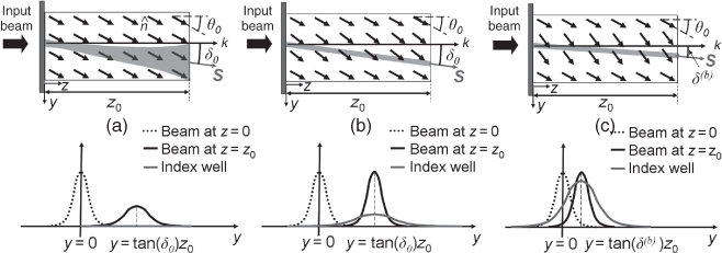
The system composed of Equations 11.1–11.4 rules the propagation of reorientational solitons in a rather general way: we can distinguish three different regimes of nematicon evolution, depending on the injected beam power. To this extent, we assume a uniform director distribution θ = θ0 in the absence of light (i.e., when A = 0) and write θ = θ0 + ψ when A ≠ 0, ψ representing the all-optical perturbation of the director. In the linear regime, that is, at very low powers, ψ is negligible in each term of Equation 11.1, including self-focusing; thus, the beam spreads according to the diffraction coefficient Dy, with energy flux at an angle ![]() with respect to
with respect to ![]() (Fig. 11.1a). As power increases, the all-optical response
(Fig. 11.1a). As power increases, the all-optical response ![]() changes, with beam self-trapping but no power-dependent trajectory: this is the nonlinear perturbative regime distinguished by ψ
changes, with beam self-trapping but no power-dependent trajectory: this is the nonlinear perturbative regime distinguished by ψ ![]() θ0 (optical reorientation negligible with respect to the unperturbed director distribution), corresponding to first-order nonlinear perturbation (Fig. 11.1b). As power increases further, ψ becomes comparable with θ0 and the all-optical term affects the trajectory of the self-confined beam: this is the nonperturbative nonlinear regime, where both beam waist and trajectory depend on light power (Fig. 11.1c). We emphasize that the ranges identifying the three regimes depend on θ0, as discussed in the following sections.
θ0 (optical reorientation negligible with respect to the unperturbed director distribution), corresponding to first-order nonlinear perturbation (Fig. 11.1b). As power increases further, ψ becomes comparable with θ0 and the all-optical term affects the trajectory of the self-confined beam: this is the nonperturbative nonlinear regime, where both beam waist and trajectory depend on light power (Fig. 11.1c). We emphasize that the ranges identifying the three regimes depend on θ0, as discussed in the following sections.
Figure 11.1 Light beam propagation in the plane yz. (a) Linear regime. (b) Nonlinear perturbative regime and (c) highly nonlinear regime.
11.2.1 Perturbative Regime
In this section, we address some general properties of nematicons in the perturbative nonlinear regime, identifying two scalar parameters able to measure nonlinearity and nonlinear walk-off as functions of the initial orientation θ0.
In the perturbative limit, the nonlinear response is not high enough to sustain narrow nematicons where Es becomes appreciable; as ψ ![]() θ0, we can substitute θ → θ0 in the leftover sinusoidal term of Equation 11.4, obtaining:
θ0, we can substitute θ → θ0 in the leftover sinusoidal term of Equation 11.4, obtaining:
where we set ![]() . Equation 11.5 is a linear Poisson equation, linking the nonlinear perturbation ψ to the beam intensity (proportional to
. Equation 11.5 is a linear Poisson equation, linking the nonlinear perturbation ψ to the beam intensity (proportional to ![]() ), which can be solved by using the Green function formalism; incidentally, such feature demonstrates the equivalence between thermal and reorientational nonlinearities in NLC in this regime [8]. After setting
), which can be solved by using the Green function formalism; incidentally, such feature demonstrates the equivalence between thermal and reorientational nonlinearities in NLC in this regime [8]. After setting ![]() , we get
, we get
with G the Green function, which takes different shapes according to the examined geometry. We stress that G rules the nonlocality: for an infinitely extended medium, the nonlinear perturbation ψ is infinitely extended because ψ resembles the electrostatic potential of a pointlike charge in empty space [18, 19]. In actual experiments, the sample size is obviously finite, implying a different G with extension defined by the closest boundaries [8, 9].
For small nonlinear perturbations we can linearize ![]() , obtaining
, obtaining ![]() (the perturbation is proportional to power, as expected), with
(the perturbation is proportional to power, as expected), with ![]() and having defined an effective (nonlocal) Kerr coefficient [12]
and having defined an effective (nonlocal) Kerr coefficient [12]
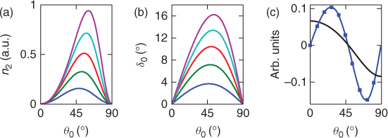
Recalling the definition of γ and considering that tanδ0∝ϵa for realistic values of the anisotropy, we find that the maximum of n2 versus θ0 is proportional to ![]() for any given K. Thus, the nonlinear behavior of an NLC mixture depends quadratically on ϵa, because of the combined effects of a stronger optical torque and a deeper index well for a fixed perturbation ψ, whereas it is inversely proportional to the elastic constant because larger K imply stronger molecular interactions counteracting the light-induced rotation. Figure 11.2a shows n2 versus θ0 for a fixed γ: all curves, each of them corresponding to a different birefringence ϵa, show a relative maximum occurring very close to θ0 = 45° for small anisotropies, moving toward higher θ0 for larger ϵa. As expected from Equation 11.7, the walk-off tanδ0 displays a similar behavior (Fig. 11.2b). Having addressed the nematicon waist with the parameter n2, we define a scalar figure cδ to describe the nematicon trajectory in the perturbative limit; it is cδ = dδ(b)/dP calculated in θ = θ0. From Equation 11.6 it is straightforward to derive
for any given K. Thus, the nonlinear behavior of an NLC mixture depends quadratically on ϵa, because of the combined effects of a stronger optical torque and a deeper index well for a fixed perturbation ψ, whereas it is inversely proportional to the elastic constant because larger K imply stronger molecular interactions counteracting the light-induced rotation. Figure 11.2a shows n2 versus θ0 for a fixed γ: all curves, each of them corresponding to a different birefringence ϵa, show a relative maximum occurring very close to θ0 = 45° for small anisotropies, moving toward higher θ0 for larger ϵa. As expected from Equation 11.7, the walk-off tanδ0 displays a similar behavior (Fig. 11.2b). Having addressed the nematicon waist with the parameter n2, we define a scalar figure cδ to describe the nematicon trajectory in the perturbative limit; it is cδ = dδ(b)/dP calculated in θ = θ0. From Equation 11.6 it is straightforward to derive
where
11.9 ![]()
Figure 11.2c shows cδ and cθ for the commercial NLC E7: the nonlinear variations in walk-off depend on the trade-off between the sensitivity of δ versus θ (parameter cθ), with absolute maxima around θ0 = 0° or θ0 = 90°, and the growth rate of θ versus power P, maximum for θ ≈ 45° and nearly zero around θ0 = 0° or θ0 = 90°. As a consequence, cδ is positive for θ0 < 48°, with a relative maximum for θ0 ≈ 26°; it is negative for θ0 > 48° and undergoes a relative minimum for θ0 ≈ 71°.
Figure 11.2 (a) Nonlinear effective coefficient n2 versus θ0 for ![]() and n|| from 1.6 (bottom line) to 2 (top line) for a constant γ. (b) Walk-off angle for
and n|| from 1.6 (bottom line) to 2 (top line) for a constant γ. (b) Walk-off angle for ![]() and n|| from 1.6 (bottom line) to 2 (top line); the NLC mixture E7 corresponds to
and n|| from 1.6 (bottom line) to 2 (top line); the NLC mixture E7 corresponds to ![]() and n|| = 1.7 in the near-infrared. (c) Graphs of cθ (solid line) and cδ versus θ0 (solid line with symbols).
and n|| = 1.7 in the near-infrared. (c) Graphs of cθ (solid line) and cδ versus θ0 (solid line with symbols).
11.2.2 Highly Nonlinear Regime
Let us consider Equation 11.4 assuming Es = 0 for simplicity; hence, ![]() . For the sake of generality, we will take θ0 to be a space-dependent function, as experimentally obtainable, for example, by defining nonuniform anchoring at the boundary (Section 5.3.2) or using patterned electrodes for the application of a low-frequency electric field (Section 5.4) [20]. When ψ becomes comparable with θ0, it is no longer possible to neglect the all-optical perturbation in the sine term, that is, the integral solution Equation 11.6 can be recast as a nonlinear integral equation
. For the sake of generality, we will take θ0 to be a space-dependent function, as experimentally obtainable, for example, by defining nonuniform anchoring at the boundary (Section 5.3.2) or using patterned electrodes for the application of a low-frequency electric field (Section 5.4) [20]. When ψ becomes comparable with θ0, it is no longer possible to neglect the all-optical perturbation in the sine term, that is, the integral solution Equation 11.6 can be recast as a nonlinear integral equation
11.10 ![]()
Setting ϵU = |A|2 (ϵ is a smallness parameter) and ![]() , a standard perturbation approach yields [8]
, a standard perturbation approach yields [8]
where we neglected all derivatives of δ with respect to θ. Equations 11.11 are an infinite set of Poisson-like equations in agreement with the Born approximation, with a forcing term depending on the perturbation U (equal to |A|2 in the limit ϵ → 1) and on the lower-order solutions. At order ϵ0, we get back the equation governing the director distribution in the absence of light. At order ϵ1, we retrieve Equation 11.5. Recalling that ![]() , in the highly nonlinear regime, the nonlinear effect ψ is no longer directly proportional to power P owing to saturation in reorientation (i.e., a complicate power series with alternating signs).
, in the highly nonlinear regime, the nonlinear effect ψ is no longer directly proportional to power P owing to saturation in reorientation (i.e., a complicate power series with alternating signs).
Let us now turn back to the case of a homogeneous θ0 and discuss these results with reference to nematicons. In Section 11.2, we defined the transition from perturbative to highly nonlinear regimes referring to the soliton trajectory, that is, comparing nonlinear changes in walk-off with its linear value δ0. From Equation 11.8 and Figure 11.2c, it is clear that the power Ptr corresponding to such transition depends on θ0 and is inversely proportional to cδ; hence, Ptr is maximum for θ0 close to 45°. Noteworthy, the higher-order terms in Equation 11.11 also affect the nematicon waist, inducing changes in the effective n2. The net result consists in a saturation of the nonlinearity, implying a nonmonotonic trend of the nematicon existence curve in the plane waist-power [21], at variance with the perturbative theories predicting a soliton waist always decreasing with power [3, 5, 22].
11.2.3 Simplified (1+1)D Model in a Planar Cell
Hereafter, we focus on homogeneous planar cells, with the shortest dimension (thickness L) along x and parallel interfaces in x = 0 and x = L. The Green function defined in Equation 11.6 reads
where we set ![]() and Ln = L/(nπ); K0 is the zeroth-order modified Bessel function of the second kind. In the framework of perturbative theories, for the sake of computational savings, in Equation 11.4 the second derivative along the Poynting vector can be neglected (this is rigorous for a soliton in bulk dielectric). This leads to several considerations: first, an a priori knowledge of the propagation direction is needed (an unknown variable in the highly nonlinear regime); second, the assumption of a zero longitudinal second derivative is equivalent to consider the medium local in this direction, an unphysical hypothesis because the Green function is radially symmetric in the plane yz (Eq. 11.12), with appreciable differences between the two models when the breathing period becomes very small; third, losses due to Rayleigh scattering are unavoidable in actual NLC samples, yielding a drop in beam power versus propagation and a weakening of the nonlinear effect, the latter resulting in a curved trajectory (via changes in δ(b)) as well as longitudinal variations of the refractive index
and Ln = L/(nπ); K0 is the zeroth-order modified Bessel function of the second kind. In the framework of perturbative theories, for the sake of computational savings, in Equation 11.4 the second derivative along the Poynting vector can be neglected (this is rigorous for a soliton in bulk dielectric). This leads to several considerations: first, an a priori knowledge of the propagation direction is needed (an unknown variable in the highly nonlinear regime); second, the assumption of a zero longitudinal second derivative is equivalent to consider the medium local in this direction, an unphysical hypothesis because the Green function is radially symmetric in the plane yz (Eq. 11.12), with appreciable differences between the two models when the breathing period becomes very small; third, losses due to Rayleigh scattering are unavoidable in actual NLC samples, yielding a drop in beam power versus propagation and a weakening of the nonlinear effect, the latter resulting in a curved trajectory (via changes in δ(b)) as well as longitudinal variations of the refractive index ![]() . Therefore, the longitudinal derivative needs to be included in the reorientational equation in order to account for all the properties of the original system (Equations 11.1 and 11.4), that is, nonlocality, self-steering and self-confinement, and their dependence on θ0 [12].
. Therefore, the longitudinal derivative needs to be included in the reorientational equation in order to account for all the properties of the original system (Equations 11.1 and 11.4), that is, nonlocality, self-steering and self-confinement, and their dependence on θ0 [12].
Numerical simulations of the full 3D model composed by Equations 11.1 and 11.4 can be carried out with standard solvers relying on iterative algorithms; the magnetic field is computed by solving Equation 11.1 (to this extent, the splitting operator can be used by choosing the Crank–Nicolson algorithm for computing diffraction); the electric field components Et and Es are calculated from Equations 11.2 and 11.3; finally, the substitution of Et and Es into Equation 11.4 allows computing the director distribution (for instance, with an over relaxed Gauss–Seidel scheme), providing the dielectric parameters for the solution of Equation 11.1. In this procedure, the relaxation code in a 3D geometry is the bottleneck on computational time.
A simplified (1 + 1)D model can be obtained by writing the all-optical perturbation in a Fourier series along x
Substituting Equation 11.13 into Equation 11.4, neglecting Es for simplicity (the generalization including the longitudinal field is straightforward) and considering a highly nonlocal response, we obtain
for every positive integer n, having exploited the orthogonality of the sine functions and having defined ![]() . Equation 11.14 is an infinite set of Yukawa equations, with the screening length in the nth equation given by L/(πn) [12].
. Equation 11.14 is an infinite set of Yukawa equations, with the screening length in the nth equation given by L/(πn) [12].
By setting A(x, y, z) = X(x, z)u(y, z) (the maximum of X is one), we get ![]() , where
, where ![]() . If we consider symmetric beams with respect to the cell midplane x = L/2 (
. If we consider symmetric beams with respect to the cell midplane x = L/2 (![]() , with |a| < L/2), light will propagate in this plane as an equal repulsion from the two parallel boundaries (placed in x = 0 and x = L) balances out (Section 11.6); moreover,
, with |a| < L/2), light will propagate in this plane as an equal repulsion from the two parallel boundaries (placed in x = 0 and x = L) balances out (Section 11.6); moreover, ![]() will be nonzero only if n is odd; hence, we can set n = 2m + 1 (m = 0, 1, 2, … ). As shown in Figure 11.3a, for a bell-shaped beam
will be nonzero only if n is odd; hence, we can set n = 2m + 1 (m = 0, 1, 2, … ). As shown in Figure 11.3a, for a bell-shaped beam ![]() is an alternating series and ψ2m+1 from Equation 11.14 has the same trend. Equation 11.13 provides
is an alternating series and ψ2m+1 from Equation 11.14 has the same trend. Equation 11.13 provides ![]() ; therefore, all terms on the right-hand side of the series have the same sign.
; therefore, all terms on the right-hand side of the series have the same sign.
Let us now analyze the propagation Equation 11.1. In the highly nonlocal limit, integrating along x yields [12]
The next step is the introduction of an equivalent two-dimensional all-optical perturbation ψ2D(y, z). Toward this goal, we set ψ2D = ψ1; thus, ψ2D is underestimated with respect to the actual ψ and we have to compensate it by an effective two-dimensional power P2D smaller than the actual power P. Defining the fit parameter σ via P = σP2D, it is σ > 1; assuming equal amplitudes of all ![]() , we get a rough estimate for σ:
, we get a rough estimate for σ:
11.16 ![]()
Figure 11.3 Fourier series of ![]() and dependence of nonlocality on the implemented model. (a)
and dependence of nonlocality on the implemented model. (a) ![]() for w/L = 0.01 (crosses), 0.05 (stars), 0.1 (circles), and 0.5 (squares), respectively. (b) Fit parameter σ versus normalized beam waist w/L. Nonlinear perturbation ψ versus y/L for the (c) Poisson and the (d) Yukawa equations when w/L = 0.05, respectively.
for w/L = 0.01 (crosses), 0.05 (stars), 0.1 (circles), and 0.5 (squares), respectively. (b) Fit parameter σ versus normalized beam waist w/L. Nonlinear perturbation ψ versus y/L for the (c) Poisson and the (d) Yukawa equations when w/L = 0.05, respectively.
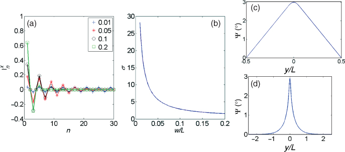
Figure 11.3b plots σ versus waist for a Gaussian beam. As expected, σ increases for narrower beams due to the spreading of In toward larger integers, as demonstrated in Figure 11.3a.
In summary, nonlinear beam propagation in NLC can be effectively modeled in (1 + 1)D by the system of Equation 11.15 and the reorientational equation
We point out that Equation 11.17 retains the degree of nonlocality of the full 3D structure. Conversely, removing the term ∂2ψ/∂2x in Equation 11.4 or 11.5 implies the disappearance of the screening term in Equation 11.17: in such case, the nonlocality range would be the cell size along y [9, 18], that is, a significant misestimate of the nonlinear index well, both in shape and size [8] (Fig. 11.3c).
11.3 Single-Hump Nematicon Profiles
In this section, we discuss light self-confinement in the absence of losses, with specific reference to single-hump nematicons; we solve the nonlinear eigenvalue problem for various powers and initial orientation θ0, comparing the results of the full 3D model with the simplified 2D model.
11.3.1 (2 + 1)D Complete Model
We consider nematicons with phase fronts normal to ![]() , that is, solitons that can be excited by beams impinging normally on the input interface of the NLC sample. Shape-preserving nonlinear wave packets will take the form A = As(x, y − tanδ(b)z)exp(ik0nNLz), and the corresponding optical perturbation is ψ = ψs(x, y − tanδ(b)z), with nNLk0 the variation induced by self-phase modulation on the propagation constant and tanδ(b) the nonlinear change in walk-off. The nonlinear eigenvalue problem has the form
, that is, solitons that can be excited by beams impinging normally on the input interface of the NLC sample. Shape-preserving nonlinear wave packets will take the form A = As(x, y − tanδ(b)z)exp(ik0nNLz), and the corresponding optical perturbation is ψ = ψs(x, y − tanδ(b)z), with nNLk0 the variation induced by self-phase modulation on the propagation constant and tanδ(b) the nonlinear change in walk-off. The nonlinear eigenvalue problem has the form
To illustrate the main properties of nonlocal spatial solitons in NLC, the system of Equations 11.18 and 11.19 can be solved in the highly nonlocal limit, that is, when the nonlocal index well can be satisfactorily approximated by a parabola. In fact, setting ![]() and neglecting tan2δ(b) with respect to 1, Equation 11.19 provides
and neglecting tan2δ(b) with respect to 1, Equation 11.19 provides ![]() , with A0 = As(x = L/2, y = 0). The beam profile is
, with A0 = As(x = L/2, y = 0). The beam profile is ![]() , where
, where ![]() (Ps is the nematicon power), and the soliton existence curve in the plane power-waist takes the expression
(Ps is the nematicon power), and the soliton existence curve in the plane power-waist takes the expression
which can be recast as ![]() .
.
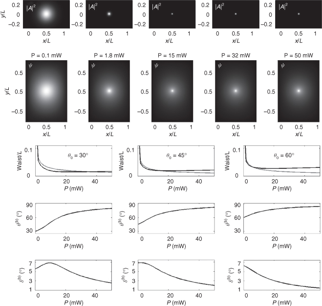
Figure 11.4 shows solutions of system (11.18 and 11.19) for θ0 = 45° versus nematicon power. At very low power, the soliton waist is comparable with the sample thickness L; hence, the nonlocality is of the order of unity and the refractive index profile is asymmetric due to the distinct boundary conditions along x (finite side) and y (infinite side). As power increases, the nematicon gets narrower because of a higher nonlinear index well; when the waist becomes much smaller than L, the highly nonlocal regime can be invoked, as confirmed by the conservation of the ψs profile versus power. For still higher powers, the soliton waist increases because of the saturation in the reorientational nonlinearity as stated by Equation 11.20, the latter also responsible for changes in soliton walk-off. Finally, consistently with Section 11.2.2, the soliton behavior with power depends on the initial angle θ0, which determines how soon saturation occurs and the angular span of soliton deflection.
Figure 11.4 Numerically calculated nematicon profiles. First (second) row: plots of the intensity |A|2 (nonlinear perturbation ψ) for several input powers and θ0 = 45°. Third row: soliton existence curve in the plane power-waist, based on the perturbation model (gray lines), and exact solution stemming from Equations 11.18 and 11.19 (black lines) for three values of θ0. Fourth (fifth) row: behavior of the maximum in director distribution θ(b) (nematicon walk-off δ(b)) versus input power for three θ0.
11.3.2 (1 + 1)D Simplified Model
Hereby, we carry out a procedure similar to the one of the former Section 11.3.1 to compute the soliton profile versus power using the simplified (1 + 1)D model described in Section 11.2.3. From Equations 11.15 and 11.17, the nematicon in the midplane x = L/2 is governed by the eigenvalue problem
Figure 11.5a shows the computed nonlinear index well ![]() at three excitations: the nonlinear reorientation ψs conserves the shape of the complete 3D model (Fig. 11.4) thanks to the presence of the screening term
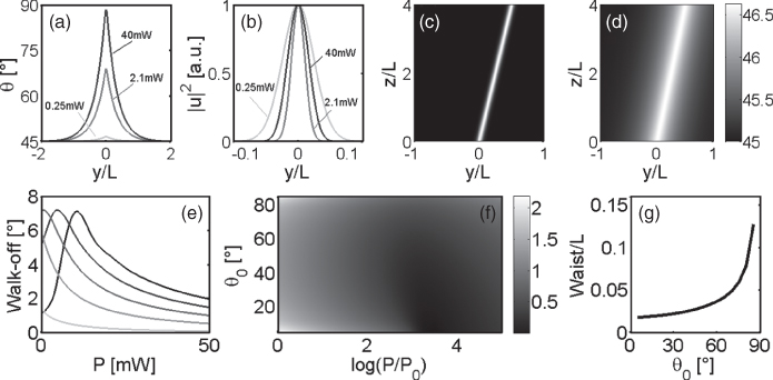
at three excitations: the nonlinear reorientation ψs conserves the shape of the complete 3D model (Fig. 11.4) thanks to the presence of the screening term ![]() , that is, the nonlocality is conserved even if the dimensionality has been reduced. The corresponding soliton profiles |us|2 are graphed in Figure 11.5b: for powers larger than 0.25 mW, the shape is very similar to Gaussian, in agreement with the highly nonlocal approximation. We checked the shape invariance of the calculated profiles by means of a bidimensional anisotropic BPM code (see Section 11.4.1 for details); the results for beam profile and director perturbation are plotted in Figure 11.5c and 11.5d, respectively. Obviously, beam self-steering due to nonlinear changes in walk-off still occurs, but its dynamics are shifted to lower powers, consistently with Section 11.2.3 (Fig. 11.5e). Furthermore, the soliton existence curve in the plane waist-power retains its nonmonotonic behavior because of saturation in the nonlinearity, although the beam dynamics versus initial condition remains the same (Fig. 11.5f). Figure 11.5g plots the minimum soliton waist for a given θ0, demonstrating that the best confinement takes place for small θ0 as it stems from the highly perturbative regime discussed in Section 11.2.2.
, that is, the nonlocality is conserved even if the dimensionality has been reduced. The corresponding soliton profiles |us|2 are graphed in Figure 11.5b: for powers larger than 0.25 mW, the shape is very similar to Gaussian, in agreement with the highly nonlocal approximation. We checked the shape invariance of the calculated profiles by means of a bidimensional anisotropic BPM code (see Section 11.4.1 for details); the results for beam profile and director perturbation are plotted in Figure 11.5c and 11.5d, respectively. Obviously, beam self-steering due to nonlinear changes in walk-off still occurs, but its dynamics are shifted to lower powers, consistently with Section 11.2.3 (Fig. 11.5e). Furthermore, the soliton existence curve in the plane waist-power retains its nonmonotonic behavior because of saturation in the nonlinearity, although the beam dynamics versus initial condition remains the same (Fig. 11.5f). Figure 11.5g plots the minimum soliton waist for a given θ0, demonstrating that the best confinement takes place for small θ0 as it stems from the highly perturbative regime discussed in Section 11.2.2.
Figure 11.5 Two-dimensional simplified model of nematicon propagation. (a) Nonlinear index well and (b) corresponding nematicon profile |us|2 computed with Equations 11.21 and 11.22. (c) Intensity profile |A|2 in yz and (d) corresponding ψ2D for P = 2.2 mW launched at the input. (e) Walk-off δ(b) versus power; from the darkest to the brightest color, θ0 ranges from 5° to 85° in steps of 20°. (f) Plot of ![]() versus power P and initial angle θ0. (g) Nematicon minimum waist versus θ0. We took w0 = 1 μm and P0 = 0.02 mW.
versus power P and initial angle θ0. (g) Nematicon minimum waist versus θ0. We took w0 = 1 μm and P0 = 0.02 mW.
11.4 Actual Experiments: Role of Losses
In Section 11.3, we computed nematicon shape and trajectory versus power and initial director angle θ0, assuming no losses in the sample. In typical experiments, the input can be controlled in profile, power, and polarization, whereas the beam evolution in yz is monitored by collecting the out-scattered light. The latter is a substantial cause of attenuation even in undoped NLC; hence, it affects actual solitons and their properties, even though many of the properties discussed in Section 11.3 hold valid (e.g., dependence of self-focusing and self-steering on θ0, nonlocality dependence on the geometry, etc.). In this section, we account for scattering losses in Equations 11.15 and 11.17, comparing the results with experimental measurements.
11.4.1 BPM (1 + 1)D Simulations
Figure 11.6 displays the numerical simulations of a Gaussian beam input with waist w0 = 5 μm propagating in NLC with attenuation α = 5 cm−1, the latter directly related to experimental measurements: for a given θ0, the beam spreads at low power (diffraction dominates over self-focusing); for increasing power, self-effects become strong enough to counteract diffraction, going from self-focusing (i.e., the waist increases more gradually than in the linear regime) to self-confinement (i.e., the waist diminishes along z). Such dynamics take place at lower powers for initial orientation θ0 close to 45°, as predicted by Figure 11.2a. At variance with the exact soliton solutions studied in Section 11.3, the beam trajectory is no longer a straight line but bends because of power attenuation along z: in fact, the perturbation ψ decays exponentially along z, thereby reducing the nonlinear walk-off. Hence, for z ![]() 1/α, the beam propagates at δ0 with respect to z, that is, the evolution goes from highly nonlinear to perturbative nonlinear regimes along z. Figure 11.7 graphs ψ corresponding to the beam in Figure 11.6. Such curves underline the differences arising in the highly nonlinear regime between the case θ0 = π/4 − Δθ and θ0 = π/4 + Δθ (0 < Δθ < π/4): in the perturbative regime, self-focusing would be of equal strength in the two cases (Fig. 11.2a), whereas at high powers, the nonlinear effects are much stronger for small θ0 than for large θ0 because of saturation when all-optical reorientation becomes comparable with the initial angle θ0. This is visible in Figure 11.8, plotting waist versus z for several θ0. As regards the trajectory, differences versus θ0 are apparent even in the nonlinear perturbative regime, as the nonlinear walk-off variations are positive (negative) when θ0 is smaller (larger) than 45° (Fig. 11.9).
1/α, the beam propagates at δ0 with respect to z, that is, the evolution goes from highly nonlinear to perturbative nonlinear regimes along z. Figure 11.7 graphs ψ corresponding to the beam in Figure 11.6. Such curves underline the differences arising in the highly nonlinear regime between the case θ0 = π/4 − Δθ and θ0 = π/4 + Δθ (0 < Δθ < π/4): in the perturbative regime, self-focusing would be of equal strength in the two cases (Fig. 11.2a), whereas at high powers, the nonlinear effects are much stronger for small θ0 than for large θ0 because of saturation when all-optical reorientation becomes comparable with the initial angle θ0. This is visible in Figure 11.8, plotting waist versus z for several θ0. As regards the trajectory, differences versus θ0 are apparent even in the nonlinear perturbative regime, as the nonlinear walk-off variations are positive (negative) when θ0 is smaller (larger) than 45° (Fig. 11.9).
Figure 11.6 Evolution of |u|2 in the plane yz, computed from Equations 11.15 and 11.17 in E7 for P = 1 μW (a), 1 mW (b), and 5 mW (c). The input waist is 5 μm, the thickness L = 100 μm, and the wavelength λ = 1064 nm.
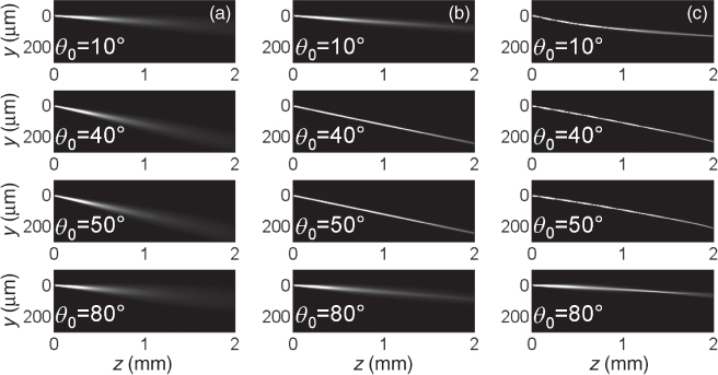
Figure 11.7 Distribution of ψ in the plane yz for P = 1 mW (perturbative regime) and P = 5 mW (highly nonlinear regime). Maxima are computed along the propagation coordinate z. Parameters are as in Figure 11.6.
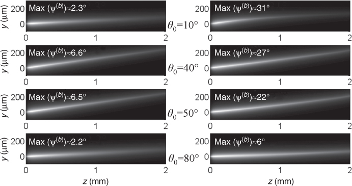
Figure 11.8 Comparison between (top) experimentally measured and (bottom) numerically calculated waist versus z. Initial θ0 are 10°, 30°, 60°, and 80°, from left to right column, respectively. The plotted values are normalized to the input waist w0. In the experimental lines, the input powers from top to bottom are 1, 2, 4, 6, 8, and 10 mW, respectively; in the simulations, they are 0.001, 0.5, 1, 3, and 5 mW, respectively.
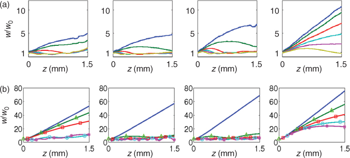
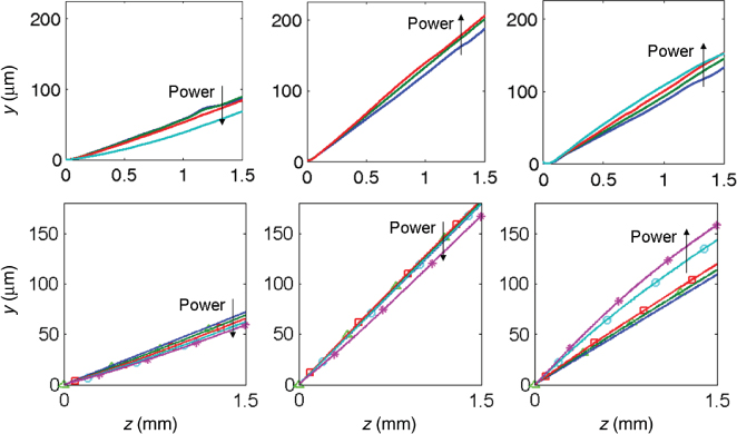
Figure 11.9 Comparison between experimentally acquired and numerically calculated trajectories. Measured (top row) and numerical (bottom row) waist versus z. Angles θ0 are 80°, 40°, and 20°, from left to right column, respectively. In the measurements, the input powers are 1, 5, and 10mW from top to bottom on the leftmost column and from bottom to top in the other two columns, respectively. The bottom (top) line in the leftmost (rightmost) column corresponds to a power of 60 mW (30 mW). The simulation powers are 0.001 mW (lines without symbols), 0.5 mW (triangles), 1 mW (squares), 3 mW (circles), and 5 mW (asterisks), respectively. Small discrepancies in the middle column are ascribable to experimental uncertainty on θ0 (most relevant in proximity to the maximum walk-off angle, see Figure 11.2b) and a different power range.
11.4.2 Experiments
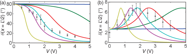
We verified our theoretical and numerical results by injecting a 5 − μm waist TEM00 beam at wavelength λ = 1064 nm in an NLC cell and observing its evolution by acquiring the image of out-scattered light (see Fig. 11.10). Two comb electrodes realized in Indium Tin Oxide are deposited on each glass–NLC interface, in order to set and tune by voltage V the angle θ0 in the midplane x = L/2; each finger of the combs is much smaller than L, ensuring a constant director angle inside the cell (Chapter 5). To quantify the dependence between θ0 and V, we measured the walk-off in the linear regime versus bias; the results are shown in Figure 11.11 (points), whereas the solid lines stem from the reorientational equation, neglecting electric field components along x and assuming an exponential decay in the applied field toward the center x = L/2 [12]. Figure 11.10 plots the acquired evolution profiles in the plane yz. As expected, at low power, the beam diffracts according to Dy, forming an angle δ0 with respect to the z-axis. As the power increases, the beam undergoes self-focusing and eventually self-confinement (top row in Fig. 11.8); self-focusing depends on θ0 and is maximum for θ0 ≈ 45°. Solitons have bent trajectories because of nonlinear changes in walk-off, with negative and positive curvatures for θ0 < 45° and θ0 > 45°, respectively, in agreement with the theoretical predictions (Fig. 11.9).
Figure 11.10 Acquired intensity profiles in the sample for various input powers and initial director angle θ0. The initial waist is 5 μm, L = 100 μm, and λ = 1064 nm.
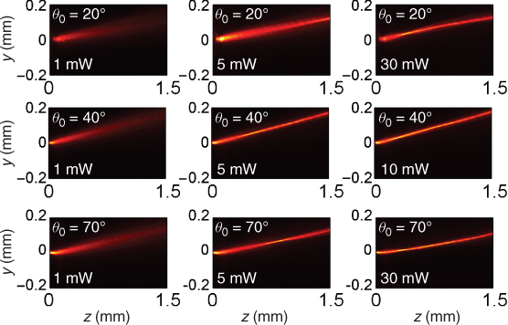
Figure 11.11 Reorientation angle in the cell midplane (a) and walk-off angle versus applied bias; points and solid lines are experimental and theoretical data, respectively. In (a) and (b), theoretical curves from left to right correspond to κ = 5 × 10⁴, 1 × 10⁵, 1.3 × 10⁵, 2 × 10⁵, 4 × 10⁵, and 2 × 10⁶ m−1, respectively.
11.5 Nematicon Self-Steering in Dye-Doped NLC
In this section, we investigate nematicons and their self-steering in dye-doped NLC. Dyes consist of molecules absorbing in a specific spectral range, altering the optical nonlinearity via the so-called Janossy effect [23, 24]. Such effect is modeled by inserting a material-dependent enhancement factor η in the expression of the optical torque; in the reorientation equation, for η > 1, the all-optical response is amplified; thus, the power can be scaled down by a factor 1/η in order to achieve the same nonlinear effects3. In this case, we consider an E7 mixture doped with 1%
in weight of 1-amino-anthraquinone (1-AAQ) [23, 25]. The input interface (placed in z = 0) is such to induce planar director orientation: at rest, the director angle θ versus z goes from θin = 90° to θ0 = 45°, the latter determined by anchoring at the two interfaces parallel to the plane yz; we also recall that the extension of the transition region along z is equal to the cell thickness L (in our case L ≈ 100 μm). Thus, we can write ![]() , being
, being ![]() the director distribution in the absence of illumination.
the director distribution in the absence of illumination.
Figure 11.12a–c shows the expected behavior on the basis of the standard Janossy effect: linear diffraction at low power, perturbative and highly nonlinear effects at higher powers, with the corresponding changes in beam waist and trajectory in analogy to the case of undoped NLC. The main difference between the doped and undoped NLC should be the lower power needed to observe nonlinear effects and the propagation losses due to dye absorption. We launched along z in the sample described above an extraordinarily polarized fundamental Gaussian beam at λ = 442.5 nm with a waist of about 5 μm. We name ϕ the angle of the Poynting vector with ![]() . The linear walk-off is nearly 9° because of the higher NLC birefringence in the blue spectrum. Losses are measured to be αdye ≈ 50 cm−1 because of the dye. Photos of the beam evolution are displayed in Figure 11.12d: clearly, the path is not as anticipated based on standard effects. Even though self-confinement takes place above a low input power of about P0 = 80 μW (i.e., η ≈ 50, consistently with values reported in literature [23]), the output slope of the self-confined waves ϕoutput (i.e., ϕ measured for z much larger than the absorption length) is not δ0, as it should in the linear limit. In particular, as power is increased, the beam gets closer to the z-axis; when P0 approaches 240 μW, we observe a thresholdlike effect with the sudden appearance of an ordinary component diffracting along z; at the same time, the extraordinary component remains self-confined but takes negative ϕoutput, the latter reaching its maximum ϕoutput = − 30° for P0 = 400 μW (Fig. 11.13a and c). Figure 11.12e shows photos of the red light (acquired through a red filter at 632.8 nm) photoemitted by the dye and eventually guided by the blue soliton; the photoluminescence is stronger corresponding to the extraordinary blue component forming a nematicon.
. The linear walk-off is nearly 9° because of the higher NLC birefringence in the blue spectrum. Losses are measured to be αdye ≈ 50 cm−1 because of the dye. Photos of the beam evolution are displayed in Figure 11.12d: clearly, the path is not as anticipated based on standard effects. Even though self-confinement takes place above a low input power of about P0 = 80 μW (i.e., η ≈ 50, consistently with values reported in literature [23]), the output slope of the self-confined waves ϕoutput (i.e., ϕ measured for z much larger than the absorption length) is not δ0, as it should in the linear limit. In particular, as power is increased, the beam gets closer to the z-axis; when P0 approaches 240 μW, we observe a thresholdlike effect with the sudden appearance of an ordinary component diffracting along z; at the same time, the extraordinary component remains self-confined but takes negative ϕoutput, the latter reaching its maximum ϕoutput = − 30° for P0 = 400 μW (Fig. 11.13a and c). Figure 11.12e shows photos of the red light (acquired through a red filter at 632.8 nm) photoemitted by the dye and eventually guided by the blue soliton; the photoluminescence is stronger corresponding to the extraordinary blue component forming a nematicon.
Figure 11.12 Expected nematicon behavior in a dye-doped NLC: for increasing power, the beam goes from (a) diffraction to (b–c) self-confinement, either in the (b) perturbative or (c) in the highly nonlinear regimes, respectively, with nonlinear response decaying exponentially in propagation owing to attenuation. (d) In actual experiments at 442.5 nm, the nematicon path and output slope depend on power, with an abrupt change in trajectory for P0 = 260 μW and the appearance of an ordinary component. (e) Images of the light emitted (and scattered) in the red portion of the spectrum, due to photoluminescence of 1-AAQ.
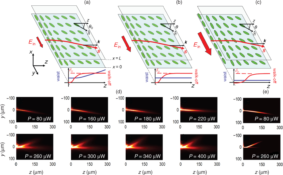
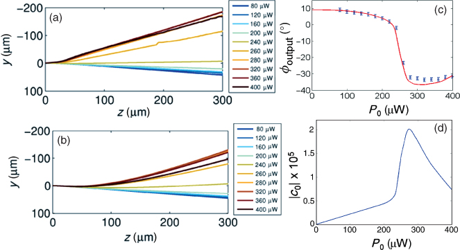
Figure 11.13 Comparison between measured trajectories and numerical results stemming from Equations 11.24 and 11.25. (a) Acquired and (b) computed nematicon trajectories; power increases from bottom to top. (c) Comparison between measured (points) and predicted (solid line) trend of the output angle ϕoutput versus power. (d) Fit coefficient c0 versus P0.
The above-described phenomena are in contrast with the hypothesis that self-bending is only caused by nonlinear changes in walk-off. In fact, they can be explained only if an effective force directed along negative y acts on the beam wave vector, thereby inducing the observed deflections even for large z. In other words, the light–matter coupling has to produce a symmetry breaking between ![]() and −
and − ![]() , consistently with the power dependence of the deflection angle.
, consistently with the power dependence of the deflection angle.
Thermal effects cannot explain the observations, given the lack of self-focusing on the ordinary component. A source of asymmetry could be the inherent anisotropy in reorientational dynamics that, for angles θ ≠ 0 and in conjunction with the boundary at the input, could misalign the beam intensity peak and the maximum of the nonlinear index well ![]() . Numerical simulations, however, confirm that, even if such effects took place, they could account for deflections up to 1°, in contrast to the experimental data. A source of asymmetry is the optical field itself: in fact, as described by Equation 11.3, in the nonparaxial regime the longitudinal field Es becomes relevant and exhibits an odd parity profile if the transverse field Et is even, as in our case. Noteworthy, solitons in doped NLC are narrow owing to the enhancement η. As the presence of Es alone is not sufficient to explain the observations, the material itself has to be sensitive to the sign of Es, that is, needs to be noncentrosymmetric. We model such noncentrosymmetry by writing
. Numerical simulations, however, confirm that, even if such effects took place, they could account for deflections up to 1°, in contrast to the experimental data. A source of asymmetry is the optical field itself: in fact, as described by Equation 11.3, in the nonparaxial regime the longitudinal field Es becomes relevant and exhibits an odd parity profile if the transverse field Et is even, as in our case. Noteworthy, solitons in doped NLC are narrow owing to the enhancement η. As the presence of Es alone is not sufficient to explain the observations, the material itself has to be sensitive to the sign of Es, that is, needs to be noncentrosymmetric. We model such noncentrosymmetry by writing
with I the intensity and Isat its saturation value. The first term on the right-hand side of Equation 11.23 accounts for saturation in the Janossy response at high peak intensities. The second term models the noncentrosymmetric response and we write Δη = c0Im(Ese−iβz), where β is the propagation constant of the self-confined wave and c0 is found by fitting the data. In the highly nonlocal limit, the soliton profile can be assumed Gaussian, that is, ![]() , where wb and yb are soliton waist and position, respectively, both of them varying with z. Under such approximations and defining the power in each section z = const as P = P0exp( − αdyez), the beam evolution can be calculated by solving the ODE system [7, 26]
, where wb and yb are soliton waist and position, respectively, both of them varying with z. Under such approximations and defining the power in each section z = const as P = P0exp( − αdyez), the beam evolution can be calculated by solving the ODE system [7, 26]
11.24 
where w0(P) is the soliton waist in the highly nonlocal and lossless (αdye = 0) case for a power P, whereas σ and χ are two constants depending on the dielectric properties of the medium [7].
The second term on the right-hand side of Equation 11.25 represents the transverse force responsible for the wave vector deviation [7]. Figure 11.13b shows the calculated trajectories: owing to losses, the wave packet self-steers in the proximity of the input interface, with paths in good agreement with the model and consistent with the change in c0 graphed in Figure 11.13d. c0 undergoes a Freedericksz-like threshold, suggesting that a torque tilts the molecular director out of the plane yz, thus explaining the appearance of the ordinary component when the sudden deviation occurs in the beam. Note that, according to the Mauguin limit, coupling between extraordinary and ordinary components can only occur for fast variations in the director distribution as compared with the wavelength: nonadiabatic variations are permitted just near the input interface, at distances smaller than the thickness L.
11.6 Boundary Effects
From Section 11.2.3–11.5, we limited ourselves to the study of nematicons propagating in the cell midplane x = L/2. Here, we discuss, both experimentally and theoretically, nematicons launched away from this plane, addressing the role of a finite cell (along x) and the consequent break in translational symmetry.
Let us consider a planar cell with director homogeneously distributed in the absence of external excitations, lying on the plane yz and forming an angle θ0 with ![]() . Assuming that the nonlinear index well conserves parity with respect to y (i.e., for an infinite sample along y), for small wave vector deviations, the application of the Ehrenfest's theorem to Equation 11.1 provides [27, 28]
. Assuming that the nonlinear index well conserves parity with respect to y (i.e., for an infinite sample along y), for small wave vector deviations, the application of the Ehrenfest's theorem to Equation 11.1 provides [27, 28]
where we set ![]() ,
, ![]() , and
, and ![]() , having defined the effective potential
, having defined the effective potential ![]() and
and ![]() . In the following discussion, we neglect nonlinear changes in walk-off in order to focus on the role played by the boundaries. In the highly nonlocal limit, in the series on the RHS of Equation 11.26, only the term for m = 0 survives, that is, the nematicon trajectory obeys geometric optics [29] (Chapter 5). To decouple the beam motion along x and in the plane yz, we exploit the separation of variables by setting |A|2/∫|A|2dxdy = φx(x, z)φy(y, z); thus, it is straightforward to get a simplified two-dimensional model for nematicon trajectory in the plane xz
. In the following discussion, we neglect nonlinear changes in walk-off in order to focus on the role played by the boundaries. In the highly nonlocal limit, in the series on the RHS of Equation 11.26, only the term for m = 0 survives, that is, the nematicon trajectory obeys geometric optics [29] (Chapter 5). To decouple the beam motion along x and in the plane yz, we exploit the separation of variables by setting |A|2/∫|A|2dxdy = φx(x, z)φy(y, z); thus, it is straightforward to get a simplified two-dimensional model for nematicon trajectory in the plane xz
where ![]() , being
, being ![]() the equivalent 1D potential. In deriving Equation 11.27, we neglected the dependence of φy on z and dropped the dependence on
the equivalent 1D potential. In deriving Equation 11.27, we neglected the dependence of φy on z and dropped the dependence on ![]() , the latter determined only by linear walk-off δ0 due to the y-invariance of the nonlinear index well.
, the latter determined only by linear walk-off δ0 due to the y-invariance of the nonlinear index well.
To complete the model, we also need an expression for the nonlinear force W0. To this extent, we use the perturbative expansion Equation 11.11 in conjunction with the Green formalism in a planar cell of finite thickness along x, as stated in Equation 11.12 for unbound geometries in yz. After the transformation y → y − ztanδ0, neglecting the partial derivatives along the propagation coordinate in the walk-off reference system of Equation 11.4, the Green function reads:
To obtain a closed form, for the nematicon we take a Gaussian ansatz, consistent with the high nonlocality [22]
11.29 
Computing the convolution integral (Eq. 11.6) employing the Green function (Eq. 11.28) provides for θ1:
with
Equation 11.30 with Equations 11.31 and 11.32 represent a closed-form solution for invariant nematicons along z propagating in planar cells, in the limit of high nonlocality and the perturbative regime, for beams launched in x = L/2 with appropriate waist (Eq. 11.20). In the more general case, these equations model a self-induced index well depending on beam position ![]() via the coefficients 11.31, that is, indicating that the nonlinear potential loses its symmetry with respect to
via the coefficients 11.31, that is, indicating that the nonlinear potential loses its symmetry with respect to ![]() when beams are not injected in the midplane x = L/2. As a consequence, the gradient of the nonlinear index center is nonzero on the beam axis, yielding a nonzero equivalent force W0 ≠ 0 on the wave packet. In the perturbative regime, we can set
when beams are not injected in the midplane x = L/2. As a consequence, the gradient of the nonlinear index center is nonzero on the beam axis, yielding a nonzero equivalent force W0 ≠ 0 on the wave packet. In the perturbative regime, we can set ![]() ; then, from Equation 11.30, we can compute Veq:
; then, from Equation 11.30, we can compute Veq:
11.33 
where we introduced ![]() , having defined the function
, having defined the function ![]() . Finally, W0 reads
. Finally, W0 reads
We stress once again that expression (11.34) was derived in the perturbative regime only for the sake of simplicity. The same derivation can be carried out considering the square terms in P stemming from ![]() and θ2 [8]; it can be found that the shape of the self-induced well (i.e., the effective force W0) is nearly unchanged owing to the high nonlocality, with the peak of the optical perturbation ψ changing by less than 10% for θ0 = 45° and P = 2 mW.
and θ2 [8]; it can be found that the shape of the self-induced well (i.e., the effective force W0) is nearly unchanged owing to the high nonlocality, with the peak of the optical perturbation ψ changing by less than 10% for θ0 = 45° and P = 2 mW.
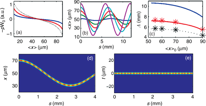
Force − pW0 versus beam position ![]() is plotted in Figure 11.14: the effective potential acting on the nematicon is anharmonic and even with respect to
is plotted in Figure 11.14: the effective potential acting on the nematicon is anharmonic and even with respect to ![]() , with the force increasing as the beam gets closer to one of the interfaces. Noteworthy, the sign of the force (negative for
, with the force increasing as the beam gets closer to one of the interfaces. Noteworthy, the sign of the force (negative for ![]() , positive or zero otherwise) is such as to repel out the beam from the boundaries, thus favoring light trapping within the NLC layer. The solutions of Equation 11.27 together with Equation 11.34 predict periodic oscillations in the nematicon trajectory; some examples are graphed in Figure 11.14b for a zero initial velocity (i.e., input beam with a zero wave vector component along x) and various input positions
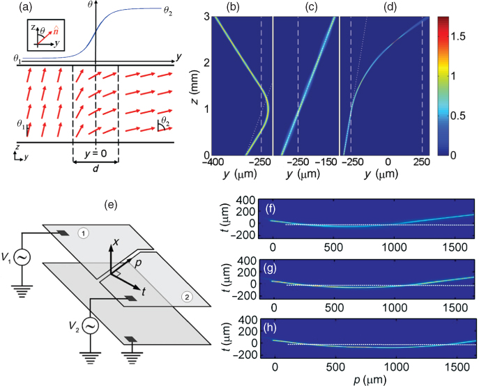
, positive or zero otherwise) is such as to repel out the beam from the boundaries, thus favoring light trapping within the NLC layer. The solutions of Equation 11.27 together with Equation 11.34 predict periodic oscillations in the nematicon trajectory; some examples are graphed in Figure 11.14b for a zero initial velocity (i.e., input beam with a zero wave vector component along x) and various input positions ![]() . The trajectory tends to a sinusoidal form in the case of small displacements from the midplane. Conversely, the oscillation period Λ decreases as the nematicon is launched further and further away from the equilibrium position x = L/2; furthermore, Λ depends on excitation because of its nonlinear origin, decreasing approximately by P−1/2 (Fig. 11.14c) [8]. We numerically simulated the PDE system of the reorientation equation and the NLSE in a 3D geometry, neglecting the second-order derivatives along the Poynting vector. We rotated the reference system xyz by δ0 around the x-axis to obtain xts. Figure 11.14d and 11.14e shows that nematicons undergo oscillations in good agreement with the theoretical predictions based on Equations 11.27 and 11.34.
. The trajectory tends to a sinusoidal form in the case of small displacements from the midplane. Conversely, the oscillation period Λ decreases as the nematicon is launched further and further away from the equilibrium position x = L/2; furthermore, Λ depends on excitation because of its nonlinear origin, decreasing approximately by P−1/2 (Fig. 11.14c) [8]. We numerically simulated the PDE system of the reorientation equation and the NLSE in a 3D geometry, neglecting the second-order derivatives along the Poynting vector. We rotated the reference system xyz by δ0 around the x-axis to obtain xts. Figure 11.14d and 11.14e shows that nematicons undergo oscillations in good agreement with the theoretical predictions based on Equations 11.27 and 11.34.
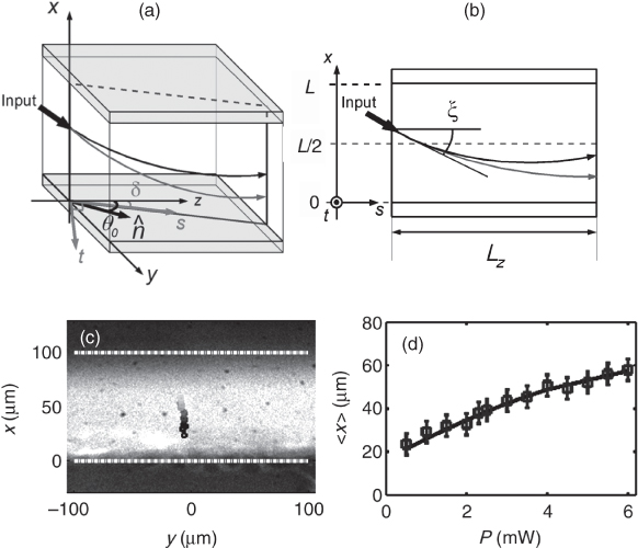
Figure 11.14 (a) Force − pW0 acting on the nematicon versus its position for excitations P = 1, 2, and 3 mW from lowest to highest (dots) absolute values, respectively. (b) Soliton trajectories in the plane xs for P = 2mW and various launch positions. (c) Oscillation period Λ (solid lines and points are theoretical predictions and numerical results, respectively) versus input position ![]() with zero initial momentum, the powers are as in (a): the largest (lowest) power corresponds to the shortest (longest) period. (d) and (e) Evolution a Gaussian beam with input waist of 2.8 μm launched in
with zero initial momentum, the powers are as in (a): the largest (lowest) power corresponds to the shortest (longest) period. (d) and (e) Evolution a Gaussian beam with input waist of 2.8 μm launched in ![]() with power 3mW and wavelength 632.8 nm in the plane (d) xs and (e) ts. Here, L = 100 μm.
with power 3mW and wavelength 632.8 nm in the plane (d) xs and (e) ts. Here, L = 100 μm.
A series of experiments were carried out to verify these findings, using an Lz = 4 − mm − long NLC cell of thickness L = 100 μm and width > 1 cm along y, with the commercial mixture E7 (Fig. 11.15a and 11.15b). The glass interfaces were treated to ensure θ0 = 30°. The soliton evolution in yz as well as the output profiles in xy (z = Lz) were imaged via CCD cameras. A small offset with respect to x = L/2 and an angular tilt ξ (in our experiments, ![]() and ξ ≈ 0.6°, respectively) were impressed on the input wave vector to maximize the nematicon x-displacement versus power; the beam at 1.064 μm was linearly polarized parallel to
and ξ ≈ 0.6°, respectively) were impressed on the input wave vector to maximize the nematicon x-displacement versus power; the beam at 1.064 μm was linearly polarized parallel to ![]() to maximize coupling to the extraordinary wave. Clearly, the soliton is expected to interact with the boundary-driven potential and oscillate for a fraction of the period Λ, shifting along x in z = Lz as power changes. The photographs of the output profiles in yz are superimposed in Figure 11.15c for several input powers (from 0.5 to 6 mW), demonstrating the predicted power-dependent repulsion from the boundary. Such nonlinear transverse dynamics along x are in excellent agreement with the integration of Equation 11.27 (using Equation 11.34 for the force) considering the actual sample parameters and a nonzero initial velocity
to maximize coupling to the extraordinary wave. Clearly, the soliton is expected to interact with the boundary-driven potential and oscillate for a fraction of the period Λ, shifting along x in z = Lz as power changes. The photographs of the output profiles in yz are superimposed in Figure 11.15c for several input powers (from 0.5 to 6 mW), demonstrating the predicted power-dependent repulsion from the boundary. Such nonlinear transverse dynamics along x are in excellent agreement with the integration of Equation 11.27 (using Equation 11.34 for the force) considering the actual sample parameters and a nonzero initial velocity ![]() , as displayed in Figure 11.15d [27].
, as displayed in Figure 11.15d [27].
Figure 11.15 (a) 3D sketch and (b) side view in plane xs of the planar cell employed in the experiments. Nematicons are launched with an initial tilt with respect to ![]() : the self-trapped beams are repelled from the interfaces, with a repulsive force increasing with power (black line corresponds to a power larger than for gray line). (c) Collected and superimposed photographs of spatial soliton profiles at the cell output plane xy for various powers, ranging from 0.5mW (darkest symbol) to 6mW (brightest symbol). (d) Experimental (squares) and calculated (solid line) output positions versus excitation. To fit the experimental data (in the presence of scattering losses), we assumed a power coupling of 50%.
: the self-trapped beams are repelled from the interfaces, with a repulsive force increasing with power (black line corresponds to a power larger than for gray line). (c) Collected and superimposed photographs of spatial soliton profiles at the cell output plane xy for various powers, ranging from 0.5mW (darkest symbol) to 6mW (brightest symbol). (d) Experimental (squares) and calculated (solid line) output positions versus excitation. To fit the experimental data (in the presence of scattering losses), we assumed a power coupling of 50%.
11.7 Nematicon Self-Steering Through Interaction with Linear Inhomogeneities
Till now, we addressed power self-steering of nematicons when they propagate in a homogeneous molecular dielectric. In this section, we discuss how dielectric inhomogeneities affect the dependence of the beam trajectory on power. We address the nonlinear Goos–Hänchen shift on TIR at an interface, that is, a power-dependent lateral beam shift at a graded interface between two nonlinear NLC regions. We also illustrate power-dependent nematicon self-ejection from a finite index well. In both cases, perturbations in director distribution are impressed via the application of suitable biases.
11.7.1 Interfaces: Goos–Hänchen Shift
Let us consider a nematicon propagating in a planar cell and encountering a dielectric interface in its path, as sketched in Figure 11.16a. We assume that the director orientation changes linearly from θ1 for y < − d/2 to θ2 for y > d/2. The transition width d has to be comparable with the shortest cell dimension L, in agreement with Equation 11.12. Figure 11.16b–d shows the results of BPM simulations, with nematicons surviving the interaction thanks to the adiabatic character of the dielectric perturbation as compared to the soliton waist. Self-confinement changes within the refractive barrier because the effective Kerr coefficient given by Equation 11.7 follows the variations in θ.
If the index contrast across the interface is high enough to provide TIR (for wave vectors along ![]() , the condition θ1 > θ2 is sufficient to ensure TIR), in the highly nonlinear regime, we expect the reflected beam path to depend on power because of nonlinear walk-off. In particular, for θ2 < θ1 < 45°, the changes in walk-off are positive (if optical powers are low enough to ensure a director angle belonging to the domain where walk-off angle is monotonically growing with θ, see Fig. 11.2c); therefore, nematicons undergoing TIR move toward positive y, giving rise to a nonlinear Goos–Hänchen shift [10].
, the condition θ1 > θ2 is sufficient to ensure TIR), in the highly nonlinear regime, we expect the reflected beam path to depend on power because of nonlinear walk-off. In particular, for θ2 < θ1 < 45°, the changes in walk-off are positive (if optical powers are low enough to ensure a director angle belonging to the domain where walk-off angle is monotonically growing with θ, see Fig. 11.2c); therefore, nematicons undergoing TIR move toward positive y, giving rise to a nonlinear Goos–Hänchen shift [10].
To verify the predictions, we performed experiments in a cell with two (top) electrodes separated by a 50 − μm gap and a common ground (bottom) electrode. Voltages V1 and V2 applied to these electrodes could lift the molecular director out of the plane yz by different amounts in the two NLC regions, defining a graded interface (Fig. 11.16e). The gap was realized in order to provide an incidence angle of 79.5° with respect to the interface normal ![]() for beams launched with wave vector along z. Although this geometry is intrinsically 3D as walk-off acts also in xz, we can use our results to qualitatively explain the nematicon behavior: when the two biases are V1 = 1.5V and V2 = 0V, the director is lifted out of the plane yz only in the first region; hence, when the soliton propagates within the graded potential, the optical torque increases the walk-off and the self-confined beam penetrates deeper inside the second region, as shown in Figure 11.16f–h, with a larger lateral shift on TIR. We stress that, for a given position and transverse velocity, the force due to the index gradient depend slightly on power as we are in the highly nonlocal case (i.e., Equation 11.27 holds valid) [12]. Finally, the beam waist is much narrower than d; thus, the asymmetry in the nonlinear index well
for beams launched with wave vector along z. Although this geometry is intrinsically 3D as walk-off acts also in xz, we can use our results to qualitatively explain the nematicon behavior: when the two biases are V1 = 1.5V and V2 = 0V, the director is lifted out of the plane yz only in the first region; hence, when the soliton propagates within the graded potential, the optical torque increases the walk-off and the self-confined beam penetrates deeper inside the second region, as shown in Figure 11.16f–h, with a larger lateral shift on TIR. We stress that, for a given position and transverse velocity, the force due to the index gradient depend slightly on power as we are in the highly nonlocal case (i.e., Equation 11.27 holds valid) [12]. Finally, the beam waist is much narrower than d; thus, the asymmetry in the nonlinear index well ![]() provoked by spatial variations of the effective Kerr effect can be neglected [30, 31].
provoked by spatial variations of the effective Kerr effect can be neglected [30, 31].
Figure 11.16 Nonlinear Goos–Hänchen shift. (a) Graph of a dielectric interface in a planar geometry. Nematicon trajectories for P = 3 mW and (b) θ1 = 60° and θ2 = 10°, (c) θ1 = θ2 = 10°, and (d) θ1 = 10° and θ2 = 70°. Dashed lines mark the graded interface boundaries, whereas dotted lines are the nematicon trajectory for θ1 = θ2 in the perturbative nonlinear regime. (e) Sketch of the double-electrode configuration exploited in the experiments. Acquired intensity profiles for (f) P = 1.6 mW, (g) 4.4 mW, and (h) 9.3 mW. The applied biases are V1 = 1.5 V and V2 = 0 V, and the wavelength is 1064 nm.
11.7.2 Finite-Size Defects: Nematicon Self-Escape
After the interaction of a nematicon with an interface, we direct our attention to a localized defect in the dielectric tensor. We consider a perturbing region invariant along z and centered in y = 0, a nematicon with wave vector parallel to the symmetry axis ![]() and initial position in y = 0. If the coefficients cδ (see Equation 11.8) corresponding to the unperturbed (i.e., in the absence of light) director distribution θ0(y) are positive, we expect the force stemming from nonlinear walk-off to be able to “push” the nematicon out of the linear trapping potential, where no restoring forces are present; thereby, above a certain excitation, the nematicon should self-escape the trap [11, 32].
and initial position in y = 0. If the coefficients cδ (see Equation 11.8) corresponding to the unperturbed (i.e., in the absence of light) director distribution θ0(y) are positive, we expect the force stemming from nonlinear walk-off to be able to “push” the nematicon out of the linear trapping potential, where no restoring forces are present; thereby, above a certain excitation, the nematicon should self-escape the trap [11, 32].
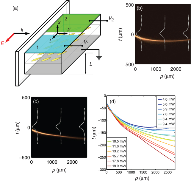
For the experiments carried out by Peccianti et al. [11], we employed the cell sketched in Figure 11.17a, similar to the one employed in Section 11.7.1 but with the two applied voltages V1 and V2 of opposite signs, in order to have the low-frequency electric field mainly in the plane yz and in the gap between the top electrodes [11]. This geometry allows us to consider molecular reorientation only in the plane yz. Figure 11.17b–d plots the experimental results: for excitations up to 4mW, the propagation in the perturbation regime allows the beam to remain trapped in the linear potential. As power is increased, the nematicon begins to bend toward positive y, until it eventually escapes the confining index well for powers larger than 13mW, as shown in Figure 11.17d.
Figure 11.17 Nematicon self-escape from a linear potential. (a) Sketch of the cell. Measured nematicon evolution in the plane tp for (b) P = 4 mW and (c) P = 13.2 mW; the dashed lines represent the (attractive) linear index well with ne peaked in y = 0. (d) Nematicon trajectories in the observation plane tp for various excitations. Here, the wavelength is 1064nm, the beam is launched in y = 0, and its initial waist is about 4 μm.
11.8 Conclusions
In this chapter, we discussed nematicon properties in the highly nonlinear regime, the latter easily accessible in NLC because of their large reorientational response. When no losses are present, nematicon evolution strongly depends on initial conditions, as we discussed with reference to saturation effects and self-steering via nonlinear walk-off. We generalized our findings to include the role of scattering losses, unavoidable in the nematic phase, and compared the theoretical predictions with experimental results. We showed how nematicons can undergo nonlinear changes in trajectory because of interaction with the boundaries, nonparaxiality and asymmetry in light–matter interaction in guest–host dye-doped NLC, interaction with inhomogeneities in the dielectric tensor. These results point out several routes toward the realization of all-optical guided-wave signal processors, allowing the design of communication networks where light itself can define and modify the topology of the implemented circuits.
Acknowledgments
Special thanks to Marco Peccianti and Malgosia Kaczmarek for their important role in the work here discussed. A.A. thanks Regione Lazio for financial support.
Notes
1 This implies that walk-off and diffraction can be assumed constant across the beam section; see Chapter 5 for details.
2 For thermo-optic effects, we should resort to the heat transmission equation; see Chapter 9.
3 Given the resonant nature of the dye, the increase in losses has to be accounted for.
1. R. W. Boyd. Nonlinear Optics. Academic Press, Boston, MA, 1992.
2. S. Trillo and S. Wabnitz. Nonlinear nonreciprocity in a coherent mismatched directional coupler. Appl. Phys. Lett., 49:752, 1986.
3. C. Conti, M. Peccianti, and G. Assanto. Route to nonlocality and observation of accessible solitons. Phys. Rev. Lett., 91:073901, 2003.
4. M. Peccianti, C. Conti, G. Assanto, A. De Luca, and C. Umeton. Routing of anisotropic spatial solitons and modulational instability in nematic liquid crystals. Nature, 432:733, 2004.
5. C. Conti, M. Peccianti, and G. Assanto. Spatial solitons and modulational instability in the presence of large birefringence: the case of highly non-local liquid crystals. Phys. Rev. E, 72:066614, 2005.
6. M. Peccianti and G. Assanto. Observation of power-dependent walk-off via modulational instability in nematic liquid crystals. Opt. Lett., 30:2290–2292, 2005.
7. A. Piccardi, A. Alberucci, and G. Assanto. Self-turning self-confined light beams in guest-host media. Phys. Rev. Lett., 104:213904, 2010.
8. A. Alberucci and G. Assanto. Propagation of optical spatial solitons in finite-size media: interplay between nonlocality and boundary conditions. J. Opt. Soc. Am. B, 24(9):2314–2320, 2007.
9. I. Kaminer, C. Rotschild, O. Manela, and M. Segev. Periodic solitons in nonlocal nonlinear media. Opt. Lett., 32(21):3209–3211, 2007.
10. M. Peccianti, G. Assanto, A. Dyadyusha, and M. Kaczmarek. Nonlinear shift of spatial solitons at a graded dielectric interface. Opt. Lett., 32:271–273, 2007.
11. M. Peccianti, A. Dyadyusha, M. Kaczmarek, and G. Assanto. Escaping solitons from a trapping potential. Phys. Rev. Lett., 101(15):153902, 2008.
12. A. Alberucci, A. Piccardi, M. Peccianti, M. Kaczmarek, and G. Assanto. Propagation of spatial optical solitons in a dielectric with adjustable nonlinearity. Phys. Rev. A, 82(2):023806, 2010.
13. M. Lax, W. H. Louisell, and W. B. McKnight. From Maxwell to paraxial wave optics. Phys. Rev. A, 11(4):1365–1370, 1975.
14. A. Alberucci and G. Assanto. Nonparaxial (1+1)D spatial solitons in uniaxial media. Opt. Lett., 36(2):193–195, 2011.
15. A. Alberucci and G. Assanto. On beam propagation in anisotropic media: one-dimensional analysis. Opt. Lett., 36(3):334–336, 2011.
16. P. G. DeGennes and J. Prost. The Physics of Liquid Crystals. Oxford Science, New York, 1993.
17. I. C. Khoo. Liquid Crystals: Physical Properties and Nonlinear Optical Phenomena. Wiley, New York, 1995.
18. C. Rotschild, O. Cohen, O. Manela, M. Segev, and T. Carmon. Solitons in nonlinear media with an infinite range of nonlocality: first observation of coherent elliptic solitons and of vortex-ring solitons. Phys. Rev. Lett., 95:213904, 2005.
19. C. Rothschild, B. Alfassi, O. Cohen, and M. Segev. Long-range interactions between optical solitons. Nat. Phys., 2:769, 2006.
20. A. Piccardi, M. Peccianti, G. Assanto, A. Dyadyusha, and M. Kaczmarek. Voltage-driven in-plane steering of nematicons. Appl. Phys. Lett., 94(9):091106, 2009.
21. A. Alberucci and G. Assanto. Nematicons beyond the perturbative regime. Opt. Lett., 35(15):2520–2522, 2010.
22. A. W. Snyder and D. J. Mitchell. Accessible solitons. Science, 276:1538, 1997.
23. I. Jánossy and T. Kósa. Influence of anthraquinone dyes on optical reorientation of nematic liquid crystals. Opt. Lett., 17(17):1183–1185, 1992.
24. L. Marrucci and D. Paparo. Photoinduced molecular reorientation of absorbing liquid crystals. Phys. Rev. E, 56:1765–1772, 1997.
25. H. Inoue, T. Hoshi, J. Yoshino, and Y. Tanizaki. The polarized absorption spectra of some α-aminoanthraquinones. Bull. Chem. Soc. Jpn., 45:1018–1021, 1972.
26. C. Conti, M. Peccianti, and G. Assanto. Observation of optical spatial solitons in a highly nonlocal medium. Phys. Rev. Lett., 92:113902, 2004.
27. A. Alberucci, M. Peccianti, and G. Assanto. Nonlinear bouncing of nonlocal spatial solitons at the boundaries. Opt. Lett., 32(19):2795–2797, 2007.
28. C. P. Jisha, A. Alberucci, R.-K. Lee, and G. Assanto. Optical solitons and wave-particle duality. Opt. Lett., 36(10):1848–1850, 2011.
29. A. Alberucci, A. Piccardi, U. Bortolozzo, S. Residori, and G. Assanto. Nematicon all-optical control in liquid crystal light valves. Opt. Lett., 35(3):390–392, 2010.
30. A. B. Aceves, J. V. Moloney, and A. C. Newell. Theory of light-beam propagation at nonlinear interfaces. i. equivalent-particle theory for a single interface. Phys. Rev. A, 39(4):1809–1827, 1989.
31. R. Barboza, A. Alberucci, and G. Assanto. Large electro-optic beam steering with nematicons. Opt. Lett., 36(14):2725–2727, 2011.
32. G. Assanto, A. A. Minzoni, M. Peccianti, and N. F. Smyth. Optical solitary waves escaping a wide trapping potential in nematic liquid crystals: Modulation theory. Phys. Rev. A, 79:033837, 2009.