
Chapter 15: Vortices in Nematic Liquid Crystals
Fenomenos Nonlineales y Mecánica, Department of Mathematics and Mechanics, Universidad Nacional Autónoma de México, Mexico D.F., Mexico
School of Mathematics and Applied Statistics, University of Wollongong , Wollongong, New South Wales, Australia
School of Mathematics and Maxwell Institute for Mathematical Sciences, University of Edinburgh, Edinburgh , Scotland, United Kingdom
School of Mathematics and Applied Statistics, University of Wollongong, Wollongong, New South Wales, Australia
15.1 Introduction
The study of optical vortices has a long history in both linear and nonlinear media. The book by Kivshar and Agrawal [1] provides a complete review of this extensive work for vortex propagation in local media. Although this extensive body of knowledge for vortex propagation in local media exists, the vortex evolution in nonlocal media, such as thermal nonlinear media and nematic liquid crystals, has been studied only recently [1]. Another recent topic of study is vortex-type structures in coupled waveguides, which provide an underlying lattice for the vortex propagation and lead to a discrete analog of a vortex [1]. It is the purpose of this chapter to describe the main analytical tools for the asymptotic analysis of the stability and propagation of optical vortices in nonlocal, nonlinear media, with an emphasis on nematic liquid crystals. To this end, we begin by recalling the basic ideas about optical vortices in the paraxial approximation, which is the limit useful for the parameter ranges for experimental studies of optical vortices in nematic liquid crystals.
In the linear limit in the paraxial approximation, the electric field E of the light of an optical vortex is described by Schrödinger's equation
Here, z is the direction of propagation and the Laplacian gives the diffractive effects in the (x, y) plane orthogonal to the direction of propagation. The initial condition at z = 0 is an input vortex experimentally produced by a mask whose thickness increases around its center by a multiple of 2π. Through the use of this mask, the rays will have a phase difference around the center of the mask, forcing the amplitude to be zero at the center and forcing circulation in the angular variable.
Elementary solutions of Schrödinger's equation (Eq. 15.1) are obtained in the form
where r and φ are polar coordinates whose origin is at the center of the mask and the function fm satisfies Bessel's equation of integer order m. The function fm(r, σ) is zero at the origin, has a maximum away from the origin, and decays to 0 at a rate r−1/2 in an oscillatory fashion. As Equation 15.1 is linear, the evolution of an initial condition
15.3 ![]()
can be obtained as a superposition in σ of the solution (Eq. 15.2). Here, m is a positive integer, termed the charge of the vortex. This representation shows that the vortex diffracts as z increases, decaying in amplitude at the rate z−1/2. In this way, the vortex beam broadens as the total power is conserved. Moreover, as happens for all solutions of the linear Schrödinger's equation, the vortex beam develops a phase that is r dependent. We thus see that vortices in linear media diffract away, as expected.
The next step is to consider the nonlinear counterpart of Equation 15.1 with a cubic nonlinearity. However, such media solutions that correspond to localized initial conditions, such as vortices, become singular in finite time [1]. This collapse behavior is avoided in saturable media [1]. For these saturable media, approximate vortex-type solutions of the form 15.2 can be determined variationally, resulting in families of vortex solutions whose width w and angular speed σ are functions of the amplitude a. It has been found that when Equation 15.2 with m = 1 is used as an initial condition for the saturable nonlinear Schrödinger (NLS) equation, it evolves into a vortex for a short distance in z and then narrows at two diagonally opposite points on the vortex. It subsequently breaks up into two lump-type beams. The spin angular momentum of the vortex is transferred to the orbital angular momentum of the beams [1]. The vortex for the saturable NLS equation is then unstable. A similar result is obtained for larger values of m. This unstable behavior is further established by solving the linearized stability problem numerically. The governing equations are linearized about the numerically found steady vortex, resulting in a linear stability problem whose eigenvalues are found numerically [2]. In this manner, it was found that there is an azimuthal instability with the fastest growing mode having wave number l = 2 for m = 1 [2]. This result explains the splitting instability of the vortex. However, this numerical analysis gives no hint of the detailed instability mechanism involved.
A first, crude argument to show the azimuthal instability in the limit of a large vortex for an NLS equation is as follows. Consider the saturable NLS equation
15.4 ![]()
where f(|u|2) approaches a constant as |u| → ∞. This equation has the Lagrangian
Here, F′(x) = f(x) and the * superscript denotes the complex conjugate. An approximate vortex solution takes the form
15.6 ![]()
where R is the radius of the vortex and the function g(ξ) is peaked around ξ = 0. Substitution of this vortex into the Lagrangian (Eq. 15.5) and integration in the radial variable gives a new Lagrangian for v(φ, z) of the form
Here,
15.8 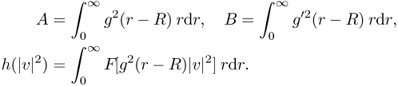
Variations of the Lagrangian (Eq. 15.7) with respect to v* show that v satisfies the one-dimensional NLS equation in the azimuthal direction
The angular part of the vortex solution then has the form
15.10 ![]()
where σ satisfies the nonlinear dispersion relation
15.11 ![]()
The expression 15.10 is a uniform wave train. It is modulationally unstable for sufficiently long-wave-sideband-type perturbations [3]. In this case, wave numbers with m = O(1) are equivalent to long wave sidebands, as the dispersion relation for the linearized equation (Eq. 15.9) shows that the effective wave number is ![]() , which is small for large R.
, which is small for large R.
The question of the behavior of the cluster of solitary waves that results from vortex destabilization has also been widely studied in local media [1]. However, in nonlocal media, the behavior of such clusters has been shown to be very different [2, 4]. In fact, in such media, the solitary wave clusters merge, forming a stable vortex that transforms orbital angular momentum into vortex spin. One question that remains to be addressed is that of the linking of the azimuthal solitary waves, which result from the numerically observed saturation of the azimuthal instabilities by the nonlocality, to suitably bifurcated branches from the basic m = 1 vortex.
Finally, it is possible to reformulate the classical problems of vortex dynamics from fluid mechanics to the context of nematic liquid crystals and then explore the results of the stabilizing effect of the nonlocality of the liquid crystal.
15.2 Stabilization of Vortices in Nonlocal, Nonlinear Media
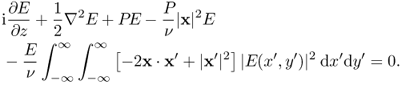
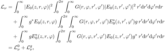
The results of the previous section show that the only way to stabilize a large vortex is to decrease the nonlinear interaction between the wave propagating around the vortex and the long-wave instability. It is clear that local media cannot decrease the size of the nonlinearity unless the medium becomes linear. However, it has been found that optical vortices can be stabilized in nonlocal, nonlinear media, as the balance required for stability is possible in such media. This stabilization in nonlocal, nonlinear media was first studied numerically by Yakimenko et al. [2] for optical vortices in nematic liquid crystals. The equations for the envelope E of the electric field of the light beam and the optical axis orientation θ of the nematic molecules are [5, 6]
The parameter ν is called the nonlocality parameter and is a measure of the elastic response of the nematic. As ν increases, the nematic becomes more nonlocal, in the sense that the response of the nematic extends (far) beyond the waist of the beam.
In the study by Yakimenko et al. [2], a steady solution of the nematic Equations 15.12 and 15.13 was sought in the form
15.14 ![]()
where f(0) = 0 and f(r) → 0 as r → ∞. The coordinates (r, φ) are the standard plane polar coordinates in the (x, y) plane. This steady solution was found by numerically solving the boundary value problem for f(r) and then finding the corresponding θ. The nematic Equations 15.12 and 15.13 were then linearized about this numerically determined steady vortex for m = 1, 2, 3, and the corresponding eigenvalue problem was solved numerically to determine the linearized stability. It was found for m = 1 that an azimuthal instability with angular dependence exp(2iφ) is present. This instability leads to the breakup of the vortex into two beams that rotate around a center and move away from each other, as illustrated in Figure 15.1. It was also shown that this instability is eliminated for large enough ν, ν ∼ 100, leading to a stable vortex. However, for m = 2 and m = 3, the corresponding instabilities with azimuthal dependencies exp(3iφ) and exp(4iφ) are not suppressed by increasing nonlocality ν. Although giving the stability picture for the nonlocal vortex, this numerical study does not give any indication of the mechanisms involved.
Figure 15.1 Numerical solution of nematicon equations (Eqs. 15.12 and 15.13) for |E| for the initial condition E = 2rexp( − r/2 + iφ), with ν = 0.5. (a) z = 0 and (b) z = 10. Source: Reproduced from Fig. 1 in Reference 4, with permission.
To study this vortex stability in a nonlocal, nonlinear nematic liquid crystal theoretically, let us use a Green's function to solve the director Equation 15.13 and then rewrite the electric field Equation 15.12 in the form
Here, K0 is the modified Bessel function of the second kind of order 0, which is the Green's function for the director Equation 15.13.
To assess the effect of the nonlocality measured by ν, let us replace the kernel K0 in Equation 15.15 by a Gaussian
15.16 ![]()
This is a commonly used kernel in studies of beam and vortex propagation in nonlocal, nonlinear media [7]. However, caution should be exercised with this Gaussian kernel, as it does not arise for any real medium [8, 9]. In particular, it does not contain the logarithmic singularity of the real kernel for a nematic liquid crystal. For this Gaussian kernel, the nonlocal term in the modified electric field Equation 15.15 can be approximated for large ν as
15.17 
For simplicity, the coordinates (x, y) have been written in the vector form x. The NLS Equation 15.15 for the electric field is then approximated by
The power
15.19 ![]()
is a conserved quantity for Equations 15.12 and 15.13 or Equation 15.15 or 15.18. We further note that the approximate Equation 15.18 for large ν is a linear Schrödinger's equation for E with harmonic oscillator and linear potentials. The approximation 15.18 is the Snyder–Mitchell approximation [10] modified by a linear potential. This linear potential can be reabsorbed into the quadratic term by a phase transformation of E. Therefore, to leading order, we can consider vortex solutions of the Snyder–Mitchell approximation [10]
15.20 ![]()
where
15.21 ![]()
Let us seek vortex-type solutions in the Snyder–Mitchell approximation 15.20
15.22 ![]()
The profile v(r) then satisfies the linear eigenvalue problem
Equation 15.23 has vortex-type solutions. The solutions with no nodes are analogs of the nonlocal vortices discussed in Reference 9. We now perturb this steady vortex by a perturbation g, so that u = u0 + g. If this perturbation does not change the power P, we have to leading order that
15.24 ![]()
Then, the linearization of the Snyder–Mitchell approximation 15.20 with u = u0 + g gives the perturbation equation
15.25 ![]()
This linear equation implies that if g is initially small, it will remain small as the solutions of this equation are bounded. Therefore, in the Snyder–Mitchell approximation, vortices are always stable. The Snyder–Mitchell approximation is then not appropriate for the study of the stability change of vortices with ν, and the full Equation 15.15 must be reexamined in detail.
To this end, let us rewrite Equation 15.15 using the additional property of the Bessel functions [12]
15.26 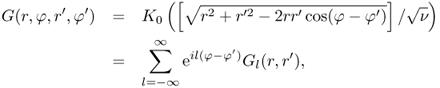
where
15.27 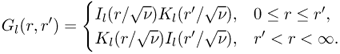
Il and Kl are the modified Bessel functions of the first and second kinds of order l. We now show how the azimuthal dependence of Green's function for the nematic Equation 15.15 can resonantly couple with the vortex with an additional azimuthal perturbation, resulting in instability. It is then necessary to study the behavior of these resonances as a function of the nonlocality. This resonant coupling can be studied using a suitable modulation theory, as detailed later.
The nonlocal Equation 15.15 has the Lagrangian density
Let us consider the m = 1 vortex, so that the trial function to obtain an approximate vortex solution is chosen to be [4]
The amplitude a and phase σ are functions of φ and z, respectively. The conjugate variables w and g are also dependent on φ and z. When the width w → 0 at a particular value of φ, the vortex is pinched at this point, which indicates that the vortex is unstable. Therefore, to examine possible instabilities, we expand w as
15.30 ![]()
Thus, as wi increases, i ≥ 1, w can become zero, leading to the breakup of the vortex. The growth of w2 will then lead to the splitting of the vortex into two beams. The shelf of radiation under the vortex given by g is also dependent on the azimuthal variable φ to take account of the distortion of the vortex due to the change of its width. The shelf of radiation g is assumed to be nonzero in the region w − R/2 ≤ r ≤ w + R/2 centered at the vortex, where the width R will be determined later.
Substituting the trial function (Eq. 15.29) into the Lagrangian (Eq. 15.28) and integrating into r from 0 to ∞ gives the averaged Lagrangian
Here, ![]() is the local contribution and
is the local contribution and ![]() is the nonlocal contribution. In detail, [4]
is the nonlocal contribution. In detail, [4]
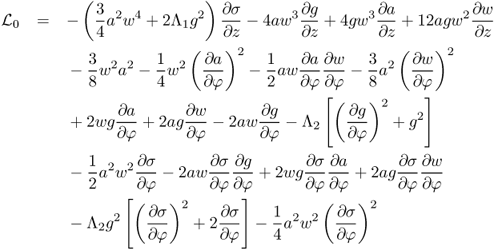
and
15.33 ![]()
The first term ![]() comes from a positive Lagrangian (Eq. 15.28), and therefore, it can only produce stable behavior under perturbations. Hence, the only destabilizing term is contained in
comes from a positive Lagrangian (Eq. 15.28), and therefore, it can only produce stable behavior under perturbations. Hence, the only destabilizing term is contained in ![]() . The quantities Λ1 and Λ2 are related to the radius of the shelf of radiation g and are given by Minzoni et al. [4]
. The quantities Λ1 and Λ2 are related to the radius of the shelf of radiation g and are given by Minzoni et al. [4]
15.34 ![]()
As remarked in the discussion after the expansion 15.27, we need to study the resonance between the vortex and the shelf g. We thus calculate ![]() to leading order, keeping only quadratic terms in g, to obtain
to leading order, keeping only quadratic terms in g, to obtain
where E0 is the vortex component and g is the shelf term of the trial function (Eq. 15.29). To calculate the first term, we note that the integral of the Green's function is just the solution of the radial equation for the director forced by ![]() . In the limit of large nonlocality ν, this forcing acts as a point source as
. In the limit of large nonlocality ν, this forcing acts as a point source as ![]() . This gives a solution that is flat where the vortex has a node, giving no contribution to the integral. The only contribution to the integral then comes from the tail and is small for ν large. We then have that
. This gives a solution that is flat where the vortex has a node, giving no contribution to the integral. The only contribution to the integral then comes from the tail and is small for ν large. We then have that
Using this result, the variational equations from the averaged Lagrangian (Eq. 15.31) give the steady-state amplitude–width relation for the vortex in the form
To examine the interaction terms, one can, in principle, substitute the Fourier expansion for g
15.38 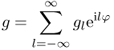
into the interaction averaged Lagrangian (Eq. 15.35) and calculate the resulting integrals approximately. However, this procedure is easier to implement on noting that the integral
15.39 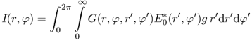
is the solution of
15.40 ![]()
This solution is regular at the origin and decays as r → ∞. Expanding I in a Fourier series gives
15.41 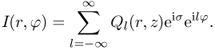
The Ql satisfy
It follows from this equation that when l ≠ 1, the solution for Ql is O(1/ν). This result could also be obtained from the exact solution for Ql in terms of Bessel functions. However, it is easier to obtain this order estimate for Ql directly from the governing Equation 15.42 by expanding the solution in powers of ν−1. The term Ql/ν then introduces an O(ν−2) correction. On the other hand, the l = 1 term can be approximated as for Equation 15.36. As the contribution of g1 is O(Λ1), the contribution is again O(ν−1) and not O(ν−1/2). It should be noted that the solution for Ql is not symmetric in l. However, the resulting averaged Lagrangian is symmetric in l due to the contribution of E0g* in expression 15.35 for ![]() . The contribution for l > 0 of the term E0g* adds with the contribution of
. The contribution for l > 0 of the term E0g* adds with the contribution of ![]() for l < 0, giving a symmetric dependence on l in the final averaged Lagrangian. The averaged Lagrangian (Eq. 15.35) then becomes
for l < 0, giving a symmetric dependence on l in the final averaged Lagrangian. The averaged Lagrangian (Eq. 15.35) then becomes
15.43 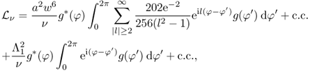
where c.c. denotes the complex conjugate of the preceding term. With this final term in the averaged Lagrangian calculated, we can now determine the stability of the vortex.
This dependence of the solution on the modes is not captured by the Snyder–Mitchell approximation. In this approximation, all the modes behave in the same manner as the nonlocal term is replaced by a radially symmetric effective potential. This difference accounts for the stable behavior of vortices in the Snyder–Mitchell approximation, whereas the full equations show that the vortices can be unstable, depending on the value of ν.
The Lagrangians ![]() and
and ![]() are then averaged with respect to the angle and z variables to obtain modulation equations for w and g. These are then linearized about the vortex fixed point given by Equation 15.37. The linearized perturbation in amplitude a is related to that in width w using the mass conservation equation. Eliminating the amplitude perturbation in this manner, we finally obtain
are then averaged with respect to the angle and z variables to obtain modulation equations for w and g. These are then linearized about the vortex fixed point given by Equation 15.37. The linearized perturbation in amplitude a is related to that in width w using the mass conservation equation. Eliminating the amplitude perturbation in this manner, we finally obtain
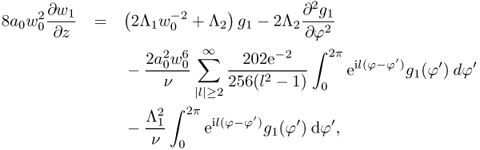
Here, the 1 subscript denotes the linear perturbation in the variable. The stability of the vortex is then reduced to the linear eigenvalue problem for the system in Equations 15.44 and 15.45. The modes are of the form
15.46 ![]()
Substitution of these modes into the system in Equations 15.44 and 15.45 results in an n-dependent system of ordinary differential equations for W and G. These ordinary differential equations have oscillatory solutions for |n| ≥ 2, provided the determinant
and a similar determinant relation for |n| = 1. From the fixed point relation 15.37, it follows that for constant steady amplitude a0, the numerator of the destabilizing term in Equation 15.47 scales as ν3/4, whereas the denominator scales as ν. It is therefore apparent that as ν becomes large, the destabilization term decays as ν−1/4, so that the vortex stabilizes for sufficiently large ν.
15.3 Vortex in a Bounded Cell
A novel experimental scenario is that in which nonlinear beams propagate in a cell for which no pretilting field is applied [13]. In these cases, the cell walls are “rubbed” to obtain a fixed orientation angle of the nematic molecules at the walls. Elastic forces then transmit this angle into the bulk of the nematic. The cell walls act as a repulsive force on a beam. This interaction with the walls can produce complicated beam trajectories, as studied using modulation theory for a nematicon (solitary wave) in References 14 and 15. The same modulation theory approach was further used to study the motion of a vortex in a finite cell [16]. In this section, we describe the main approximations used to study optical vortices in finite cells and use modulation theory to qualitatively predict the motion of vortices under different conditions.
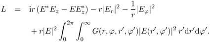
In the absence of a pretilting static electric field, the equations governing a vortex in a nematic cell are
Here, E is the electric field of the optical beam and θ is the deviation of the optical director from its initial pretilt angle due to rubbing. These equations hold in some region Ω in the transverse (x, y) variables with θ = 0 on the boundary of Ω. Poisson's equation (Eq. 15.49) can be solved for θ using a Green's function G. On substituting this solution for θ into Equation 15.48, we obtain a single equation for the electric field E, which has the Lagrangian
where
15.51 ![]()
The kernel G(x, x′) is the Green function for the Poisson's equation (Eq. 15.49) in Ω, with source x′ and G(x, x′) = 0 for x on the boundary of Ω.
Let us assume that the nonlocality ν is large so that a vortex is stable [2]. We shall assume a trial function for E to be of the form
The amplitude a and width w are taken to satisfy the amplitude–width relation for a steady vortex, which will be determined. The position X(z) = (X(z), Y(z)) and velocity V(z) of the vortex are given by the Euler–Lagrange equations obtained by substituting the trial function (Eq. 15.52) into the Lagrangian (Eq. 15.50) and then averaging.
The determination of the Green's function G is, in principle, standard. However, there are a few closed-form expressions for G that can be used to understand, in simple terms, the motion of the vortex. The simplest instance for which the Green's function can be explicitly determined is Ω being the half space y > 0. In this case, the method of images provides the desired Green's function with only one image point. In fact, the fundamental solution for the whole space − ∞ < x, y < ∞ is
15.53 ![]()
where x′ = (ξ, η) being the source. For the half space y > 0, the image is located at ![]() . The Green's function for the half space is then
. The Green's function for the half space is then
where
15.55 ![]()
This Green's function is then used to calculate the averaged Lagrangian. This cannot be done explicitly. However, the integrals can be approximated if we assume that the scale of variation of the vortex is small compared with that of the director field. In this case, we can use the approximation
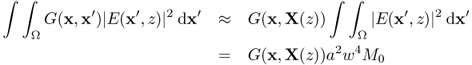
on using the trial function (Eq. 15.52). The integral M0 is
15.57 ![]()
The assumption that the size of the region Ω is much larger than the width w of the vortex has been made to extend the limit of integration in M0 to ∞.
In the case of the half space y > 0, with the Green's function being given by Equation 15.54, the nonlinear term, that is, Equation 15.56, is
15.58 ![]()
where ![]() . The corresponding term in the averaged Lagrangian is then
. The corresponding term in the averaged Lagrangian is then
15.59 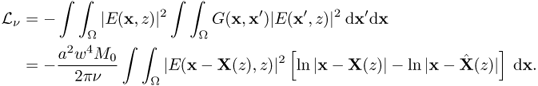
Changing variables using ![]() and then assuming that the region Ω is large compared with the size of the vortex results in, after changing to polar coordinates,
and then assuming that the region Ω is large compared with the size of the vortex results in, after changing to polar coordinates,
The second term in ![]() arises from approximating the Green's function by its value at the vortex center. The integral M1 is
arises from approximating the Green's function by its value at the vortex center. The integral M1 is
15.61 ![]()
The remaining terms in the averaged Lagrangian are calculated as in Section 15.2. The final averaged Lagrangian for the half space y > 0 is then
15.62 ![]()
where ![]() given by
given by
15.63 ![]()
and ![]() is given by Equation 15.60.
is given by Equation 15.60.
We have assumed that the vortex is small compared with the size of the cell and that its motion is slow. Let us further assume that it is far from the cell walls. In this case, the variational equations for a and w decouple from those for the position and velocity of the vortex. Variations with respect to a and w give the amplitude–width relation for a steady vortex as
This steady vortex relation is different from that, expression 15.37, which applies when there is an external biasing electric field. To simplify the analysis and resulting equations, let us assume that the vortex profile is in its equilibrium shape given by the amplitude–width relation (Eq. 15.64). In effect, we are assuming that the time evolution of the amplitude and width of the vortex are slow compared to its motion. A similar assumption was made in Chapter 7. Under this assumption, variations with respect to V and X give the position of the vortex being determined by
The potential in the last equation of Equation 15.65 is then infinitely repulsive at the cell wall. Therefore, if a vortex travels toward the wall, it is bounced back away from it. The component of the motion parallel to the wall is not altered by the image. This scenario is different from that of a vortex in an ideal fluid, which can move parallel to a wall with a velocity that depends on its strength [17].
We then expect that a vortex, or a beam, in a closed cell will be repelled by the walls and will reach an equilibrium position due to momentum being shed in diffractive radiation as it evolves [16, 18]. We now show that this is indeed the case.
Mathematically, the simplest possible closed cell is a circular cylinder of radius R. In this case, the regular part of the Green's function is [19]
15.66 
Using this representation and the fact that the vortex is assumed to be much smaller than the circular cell, w ![]() R, we can approximate the integral for
R, we can approximate the integral for ![]() as before to obtain
as before to obtain
15.67 ![]()
The final averaged Lagrangian is then ![]() . The repulsive nature of the cell boundary |X(z)| = R is clear.
. The repulsive nature of the cell boundary |X(z)| = R is clear.
In the simple case with no angular velocity X = (x(z), 0), V = (p(z), 0), the equation of motion obtained from the variational equations for the averaged Lagrangian is the oscillator equation
15.68 ![]()
This equation shows the oscillatory motion of the vortex about the center of the cell due to the repulsion of the cell walls. The vortex will eventually settle to the center of the cell due to the effect of radiation loss.
The case when the vortex has angular momentum is analyzed using polar coordinates r = |X| and polar angle φ. It is then found that the equations for the trajectory of the vortex can be expressed in the Kepler form
15.69 ![]()
The angular momentum ![]() is then a conserved quantity. Equation 15.70 shows that the origin is repulsive, as is the cell wall r = R. Equation 15.70 has bounded solutions that oscillate in the radial variable about the fixed point rf, with
is then a conserved quantity. Equation 15.70 shows that the origin is repulsive, as is the cell wall r = R. Equation 15.70 has bounded solutions that oscillate in the radial variable about the fixed point rf, with
15.71 ![]()
for R ![]() w, and that advance in the angular direction with angular velocity
w, and that advance in the angular direction with angular velocity
15.72 ![]()
Again, loss to shed diffractive radiation will decrease the angular momentum and the vortex will then slowly spiral into the center of the circular cell.
Arbitrary closed, smooth regions, Ω, can be mapped onto a circle via conformal mapping [20]. Even if this mapping is not explicit, some general qualitative statements can be made about the motion of a vortex. The Green's function H for a region Ω takes the form
15.73 ![]()
where f(z), z = x + iy, and maps the region Ω into the interior of the circle, with G being the Green's function for the circle. Therefore, the potential for the motion of the vortex, which is the regular part R of the Green's function, has as level lines in Ω the images of circles under the inverse mapping of f(z). The center of the circle is mapped to a point z0 in Ω. The vortex is then bounced away from the cell walls, the boundary of Ω, until it eventually settles in equilibrium at z0.
A rectangular or polygonal region Ω can be explicitly mapped onto the half plane using the Schwarz–Christoffel map and then onto the circle [20]. Although the conformal map is not explicit in general, the qualitative behavior of the vortex is as before—it settles to the center of the cell. For the special case of a rectangular cell, the motion of the vortex can be approached in a different manner. Green's function can be found using a Fourier series, which is then summed using Poisson's formula, resulting in a solution in terms of infinitely many images [15]. These images are placed on a lattice obtained by periodically extending the region Ω and reflecting the Green's function source in each wall [15]. To ensure the zero-boundary condition, the images have alternating signs. This image solution explains qualitatively why the motion of an optical vortex near a corner in the domain Ω is more complicated due to the influence of an infinite series of images, which has a small effect on the motion away from the corner.
In principle, one can formulate nematic vortex problems as for the classical vortices of perfect fluid flow [17]. However, the corresponding solutions will not be the same as those for fluid flow, as already seen earlier for a single nematic vortex close to an infinite straight wall.
15.4 Stabilization of Vortices by Vortex–Beam Interaction
In saturable media, the interaction between a dark vortex and a beam has been studied [1, 21]. Using two wavelengths (colors) of coherent light, a beam or vortex in one color can interact with a beam or vortex in another color [22]. The interaction between these two colors can have a significant effect on the evolution of the beams and/or vortices. For instance, it has been shown that a dark vortex in one color can form a waveguide for a beam in another color [1, 21]. In this work, the interaction of a bright vortex with a bright beam in another color was not considered, as bright vortices are unstable in local media. However, bright vortices are stable in nonlocal media, such as a liquid crystal, for sufficiently large nonlocality [2]. The interaction of an m = 1 vortex with a beam was studied by Yakimenko et al. [2]. Subsequently, an asymptotic theory was developed, which showed that a beam can stabilize a bright vortex in a nematic liquid crystal, with the stability region greatly enlarged to ν ≥ O(10) [23, 24]. Let us now consider the main ideas of this analysis.
As in the previous section, the equations governing a beam in one color (wavelength) u and a vortex in another color (wavelength) v are [22–24]
15.74 ![]()
15.75 ![]()
A slightly different scaling of these equations has been used from that in the previous section. Also, the diffraction coefficients Du and Dv and the coupling coefficients between the light and the nematic Au and Av have been left general, rather than both being scaled to 1. In experiments, these coefficients are very close. For instance, in the experiments of Alberucci et al. [22], the diffraction coefficients are 0.805 for red light and 0.823 for near-infrared light. The Lagrangian for the two color equations (Eqs. 15.74–15.76) is
As the diffraction and coupling coefficients differ by only a few percent, the simplifying assumption Du = Dv = 1 and Au = Av = 1 will be made.
The numerical results displayed in Figure 15.2 show that the beam in the second color stabilizes the vortex even for the low value ν = 4 of nonlocality. It is clear from the figure that the width of the stabilized vortex is larger than that of the supporting beam (nematicon). We recall from the previous section that a vortex is stabilized for large ν by the relatively large deformation of the optical axis in its center. It is then plausible to expect stabilization of a vortex if the optical axis in its core is deformed by a beam in the other color. Let us now verify this qualitative picture with a modulation analysis.
Figure 15.2 Numerical solution of two-color equations (Eqs. 15.74–15.76) for the initial condition (15.79 and 15.80) with g = 0. (a,b) Input and output intensities for an unstable vortex in color v with no beam in color u. (c,d) Vortex in color v (c) stabilized by nematicon in color u (d). Here, ν = 4. Source: Reproduced from Fig. 1 in Reference 24, with permission.
We see from the stability result (Eq. 15.47) that the destabilizing term for a single-color vortex is
This destabilizing term decreases as ν increases and as w0 decreases. Numerical results show that for a two-color vortex–beam pair, as the vortex stabilizes, the width of the vortex decreases because of the effect of the beam in the other color. To determine the stability of the vortex analytically, we then need to calculate the effect of the beam on the width of the vortex and show that its width decreases as the beam amplitude increases.
Suitable trial functions for the beam and an m = 1 vortex are
15.79 ![]()
15.80 ![]()
with the director being given by
15.81 ![]()
Here, (r, φ) are the polar coordinates based on the center of the vortex. Substituting these trial functions into the Lagrangian (Eq. 15.77) and averaging by integrating in r from 0 to ∞ and φ from 0 to 2π gives the averaged Lagrangian
15.82 ![]()
Here, ![]() is the contribution due to the beam,
is the contribution due to the beam, ![]() is the contribution due to the vortex, and
is the contribution due to the vortex, and ![]() is the interaction-averaged Lagrangian. From the work of the previous sections,
is the interaction-averaged Lagrangian. From the work of the previous sections, ![]() is given by Equation 15.32 and
is given by Equation 15.32 and ![]() is given by Equation 15.35. It is then only necessary to calculate the interaction term
is given by Equation 15.35. It is then only necessary to calculate the interaction term ![]() . This term is responsible for the change in the steady amplitude–width relation for the vortex from that given by Equation 15.37.
. This term is responsible for the change in the steady amplitude–width relation for the vortex from that given by Equation 15.37.
The numerical solution of Figure 15.2 shows that the vortex is stabilized by the beam in the second color, and this stabilization is accompanied by a decrease in the vortex's width. We therefore need to estimate the decrease in the width of the vortex as a result of its interaction with the beam in the second color. To this end, we consider the Lagrangian (Eq. 15.77) and average the interaction term in this Lagrangian to obtain
15.83 ![]()
This interaction term can be rearranged by integrating by parts and using the symmetry of Green's function for the director Equation 15.76 to obtain
15.84 ![]()
To calculate θv, we use the same approximations as used to derive the averaged Lagrangians 15.35 and 15.36 in Section 15.2. These approximations assume that the v color vortex is narrow in comparison with ![]() , which is the size of the width of the director field. The equation for θv in this limit of
, which is the size of the width of the director field. The equation for θv in this limit of ![]() can be approximated as
can be approximated as
15.85 ![]()
15.86 ![]()
This equation has the solution
15.87 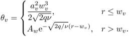
For θv to be continuous, we have
15.88 ![]()
The interaction averaged Lagrangian is then
15.89 ![]()
The interaction of the vortex with the beam is weaker than the self-interaction of the beam. We can then use the steady-state amplitude–width relation for an isolated beam [25]
15.90 ![]()
Here,
15.91 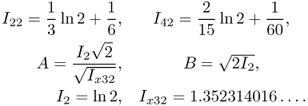
Taking variations of the resulting averaged Lagrangian with respect to av and wv then gives the steady-state amplitude–width relation
15.92 ![]()
where
15.93 ![]()
Clearly, as the beam power ![]() , we recover the amplitude–width relation (Eq. 15.37) for a free vortex, once the different scalings of the single-color Equations 15.12 and 15.13 and the two-color Equations 15.74–15.76 are accounted for. However, as the power
, we recover the amplitude–width relation (Eq. 15.37) for a free vortex, once the different scalings of the single-color Equations 15.12 and 15.13 and the two-color Equations 15.74–15.76 are accounted for. However, as the power ![]() of the beam increases, we have
of the beam increases, we have
15.94 ![]()
which gives the narrowing of the vortex by the beam, as observed in numerical solutions. This beam interaction and narrowing causes the vortex to be stable for smaller ν than for a free vortex, as the destabilizing term in Equation 15.78 becomes smaller. Minzoni et al. [24] showed that this modulation analysis gave a stability threshold in excellent agreement with the numerical threshold of ν = 5, which is much lower than the threshold ν ∼ 100 for an isolated vortex [2, 4].
It is expected that this mechanism of stabilization by a beam in another color will be able to stabilize other types of coherent structures that are unstable at relatively low values of nonlocality ν. In the following section, the stabilization mechanism for azimuthally dependent vortices is explored numerically. This study again shows the effectiveness of a beam in another color in stabilizing more complicated structures.
15.5 Azimuthally Dependent Vortices
Let us now consider the evolution of vortex-like initial conditions of the form
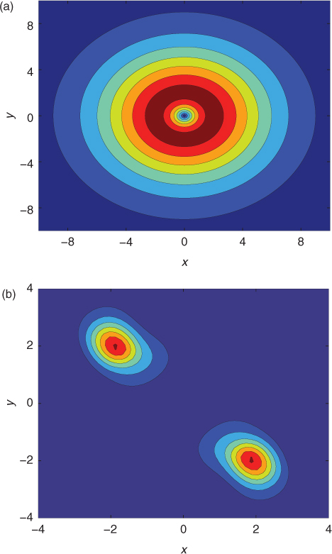
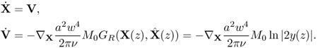
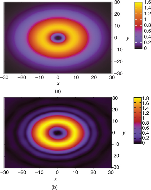
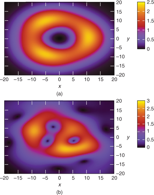
The appropriate governing equations are now Equations 15.12 and 15.13, as the nematic is pretitled by a static external electric field. These vortices were considered by Yakimenko et al. [2] and were found to be unstable for ν values of up to 200. The instability for ν < 200 manifests itself by the vortex breaking up into m + 1 lumps, which rotate in a circular motion. The radius of the circle becomes larger as z increases, with the motion of the individual lumps becoming slower. A typical unstable example is shown in Figure 15.3. A modulation theory analysis of this vortex evolution predicts that for sufficiently large ν values, the vortex is stable. To test this prediction, the nematicon Equations 15.12 and 15.13 were solved for ν = 400 and a vortex with m = 3 was found to be stable up to z ∼ 400, which is a typical nondimensional length of a nematic cell [11]. This stable vortex evolution is shown in Figure 15.4.
Figure 15.3 Solution of Equations 15.12 and 15.13 for |E| for the initial condition 15.95, with a = 0.02 and w = 3.0 for m = 3 and ν = 5. (a) z = 0 and (b) z = 50.
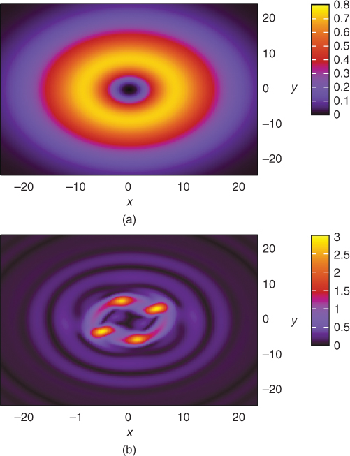
Figure 15.4 Solution of Equations 15.12 and 15.13 for |E| for the initial condition 15.95, with a = 0.04 and w = 3.0 for m = 3 and ν = 400. (a) z = 0 and (b) z = 400.
It has also been shown that a collection of beams rotating in a circle merges into a vortex when the nonlocality ν is large due to the overlap of the radiation shelves generated by each beam as it evolves [26]. Skupin et al. [7] showed that azimuthally dependent vortices exist for suitably chosen parameter values in the infinite nonlocality limit put forth by Snyder and Mitchell [10]. These vortex solutions have rectangular shapes that rotate around a dark center and were termed azimuthons.
We now describe the role of these azimuthons in the transition from a vortex to a cluster of beams rotating around a common center. Let us take the specific case m = 3. The azimuthal instability with mode n = 3 for the m = 3 vortex (Eq. 15.95) is responsible for shrinking the vortex width in the form w = w0 + w3cos3φ, with instability occurring as w3 increases. However, in principle, it is possible for the instability to saturate. If such a saturation occurs, the maximum of the vortex amplitude in the radial variable will be at
15.96 ![]()
This is the polar equation of the corresponding level line, which is triangular. To test this possibility, an initial condition with triangular level lines and a vortex angular dependence was used, this being
where R(φ) = r0 + bcos3φ. The nematicon equations (Eqs 15.12 and 15.13), which apply when there is a pretilting external electric field, and Equations 15.48 and 15.49, which apply when there is no pretilting electric field, were then solved numerically for this initial condition. Under both operating conditions, it was found that azimuthons are unstable and broke up due to a parametric instability. An example of an unstable one-color azimuthon is shown in Figure 15.8, where it forms part of the following discussion of two-color azimuthon and beam vector solitary waves.
Finally, the instability mechanism was also tested using a stabilizing beam in a second color. In this case, the equations governing a beam in one color (wavelength) u and a vortex in another color (wavelength) v are [22–24]
15.98 ![]()
15.99 ![]()
15.100 ![]()
In these governing equations, the simplifying assumption that the diffraction and coupling coefficients for each color are equal has been made. As discussed in Section 15.4, these coefficients only differ by a few percent points in experiments. The initial condition for v is Equation 15.97, and the initial condition for u is
15.101 ![]()
Figures 15.5, 15.6, 15.7 show the change of stability of the azimuthon as the nonlocality ν increases. For low values of ν, the azimuthon shows the typical vortex instability and it breaks up into beams (Fig. 15.5). As the nonlocality increases, the azimuthon becomes stable for longer distances and shows more complicated breakup behavior (Fig. 15.6). Finally, for very large values of the nonlocality, the azimuthon is stable for typical cell lengths (Fig. 15.7). It should be noted, however, that the values of the nonlocality ν for which the azimuthon is stable over a cell length are much larger than typical experimental values [11]. The vital role of the second color beam in stabilizing the azimuthon is illustrated in Figure 15.8. Comparing Figures 15.7 and 15.8 shows that the azimuthon is stable for ν = 1000 in the presence of a second color beam, but is unstable for this large nonlocality in the absence of the beam.
Figure 15.5 Solution of two-color equations (Eqs. 15.98–15.100) for |v| for the initial conditions 15.97 and 15.101, with av = 0.01, wv = 6.0, au = 1.5, wu = 5.0. r0 = 1.0, b = 0.5, and ν = 100. (a) |v| at z = 0 and (b) |v| at z = 400.
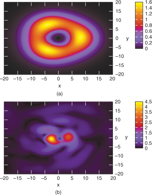
Figure 15.6 Solution of two-color equations (Eqs. 15.98–15.100) for |v| for the initial conditions 15.97 and 15.101, with av = 0.01, wv = 6.0, au = 1.5, wu = 5.0. r0 = 1.0, b = 0.5, and ν = 200. (a) |v| at z = 0 and (b) |v| at z = 400.
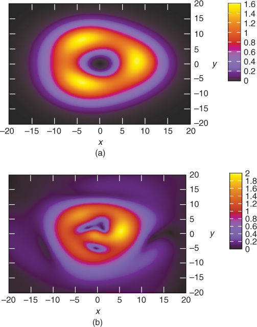
Figure 15.7 Solution of two-color equations (Eqs. 15.98–15.100) for |v| for the initial conditions 15.97 and 15.101, with av = 0.007, wv = 8.0, au = 1.5, wu = 5.0. r0 = 1.0, b = 0.5, and ν = 1000. (a) |v| at z = 0 and (b) |v| at z = 400.
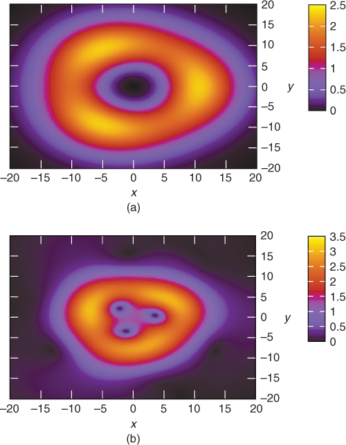
Figure 15.8 Solution of two-color equations (Eqs. 15.98–15.100) for |v| for the initial conditions 15.97 and 15.101, with av = 0.007, wv = 8.0, au = 0.0, wu = 5.0. r0 = 1.0, b = 0.5, and ν = 1000. (a) |v| at z = 0 and (b) |v| at z = 400.
Finally, in a recent work, it was shown that guided azimuthally, dependent modes can become azimuthons in a nonlinear, nonlocal medium [27]. In this context, it is of interest to consider the influence of an external voltage bias, such as considered by Assanto et al. [11], on the behavior of azimuthons in liquid crystals.
15.6 Conclusions
As well as solitary wave beams, nematicons, nematic liquid crystals can support the propagation of optical vortex beams. In local media, such optical vortices are unstable due to a dominant azimuthal n = 2 instability that splits the vortex into two solitary wave beams. However, a nematic liquid crystal is a nonlocal, nonlinear medium, and the nonlocal nature of the interaction of the optical field with the nematic stabilizes the vortex, as long as the nonlocality ν is sufficiently large. This stabilization effect of the nematic, or optical axis, on a vortex is most dramatically revealed through the interaction of a nematicon with a copropagating vortex. The nematicon deforms the optical axis, that is, makes the director rotation nonzero, at the center of the vortex, thus stabilizing it. This stabilization effect of the copropagating nematicon reduces the stability threshold for the vortex in the nonlocality ν by a factor of 10. Copropagating nematicons can be used to stabilize other vortex structures. For example, azimuthons, vortices with azimuthal structure, are stabilized by a copropagating nematicon. Indeed, a copropagating nematicon allows these azimuthally dependent structures to take complicated forms.
The analysis of the propagation of vortices in a finite nematic cell is more complicated than that in an infinite cell because of the necessity of the director satisfying anchoring conditions. The same general conclusion that nonlocality stabilizes a vortex also holds. A neglected technique that has been shown to be useful for finite cells is the method of images [15]. The advantage of this technique is that it allows the anchoring conditions for the nematic to be incorporated in a mathematically simple manner. The method of images has been exploited extensively in the fluid mechanics literature, and many of the solutions hence derived could be transferred over to the nonlinear optics of nematicons and vortices.
Azimuthally dependent vortices can be obtained, in principle, as bifurcating structures due to the development of azimuthal instabilities. An analytical description of this bifurcation requires a trial function that incorporates both the evolution of the instability and the modulation of the shape of the vortex. This is an unresolved problem.
Acknowledgments
This research was supported by the Royal Society of London under Grant No. JP090179.
1. Y. S. Kivshar and G. Agrawal. Optical Solitons: From Fibers to Photonic Crystals. Academic Press, San Diego, CA, 2003.
2. A. I. Yakimenko, Y. A. Zaliznyak, and Y. S. Kivshar. Vortex solitons in nonlocal self-focusing nonlinear media. Phys. Rev. E, 71:065603, 2005.
3. G. B. Whitham. Linear and Nonlinear Waves. John Wiley & Sons, New York, 1974.
4. A. A. Minzoni, N. F. Smyth, A. L. Worthy, and Y. S. Kivshar. Stabilization of vortex solitons in nonlocal nonlinear media. Phys. Rev. A, 76:063803, 2007.
5. C. Conti, M. Peccianti, and G. Assanto. Route to nonlocality and observation of accessible solitons. Phys. Rev. Lett., 91:073901, 2003.
6. C. Conti, M. Peccianti, and G. Assanto. Observation of optical spatial solitons in a highly nonlocal medium. Phys. Rev. Lett., 92:113902, 2004.
7. S. Skupin, M. Grech, and W. Krolikowski. Rotating soliton solution in nonlocal nonlinear media. Opt. Express, 16:9118–9131, 2008.
8. Z. Xu, Y. V. Kartashov, and L. Torner. Upper threshold for stability of multipole-mode solitons in nonlocal nonlinear media. Opt. Lett., 30:3171–3173, 2005.
9. S. Skupin, O. Bang, D. Edmundson, and W. Krolikowski. Stability of two-dimensional spatial solitons in nonlocal nonlinear media. Phys. Rev. E, 73:066603, 2006.
10. A. W. Snyder and M. J. Mitchell. Accessible solitons. Science, 276:1538–1541, 1997.
11. G. Assanto, A. A. Minzoni, M. Peccianti, and N. F. Smyth. Optical solitary waves escaping a wide trapping potential in nematic liquid crystals: modulation theory. Phys. Rev. A, 79:033837, 2009.
12. M. Abramowitz and I. A. Stegun. Handbook of Mathematical Functions with Formulas, Graphs and Mathematical Tables. Dover Publications, New York, 1972.
13. Q. Shou, Y. Liang, Q. Jiang, Y. Zheng, S. Lan, W. Hu, and Q. Guo. Boundary force exerted on spatial solitons in cylindrical strongly nonlocal media. Opt. Lett., 34:3523–3525, 2009.
14. A. Alberucci, G. Assanto, D. Buccoliero, A. Desyatnikov, T. R. Marchant, and N. F. Smyth. Modulation analysis of boundary induced motion of nematicons. Phys. Rev. A, 79:043816, 2009.
15. A. A. Minzoni, L. W. Sciberras, N. F. Smyth, and A. L. Worthy. Propagation of optical spatial solitary waves in bias-free nematic liquid crystal cells. Phys. Rev. A, 84:043823, 2011.
16. A. A. Minzoni, N. F. Smyth, and Z. Xu, Stability of an optical vortex in a circular nematic cell. Phys. Rev. A, 81:033816, 2010.
17. H. Lamb. Hydrodynamics. Dover Publications, New York, 1945.
18. G. Assanto, C. García-Reimbert, A. A. Minzoni, N. F. Smyth, and A. L. Worthy. Lagrange solution for three wavelength solitary wave clusters in nematic liquid crystals. Physica D, 240:1213–1219, 2011.
19. R. Courant and D. Hilbert. Methods of Mathematical Physics, Vol. 1. Interscience Publishers, New York, 1965.
20. M. J. Ablowitz and A. S. Fokas. Complex Variables. Introduction and Applications. Cambridge University Press, Cambridge, 1997.
21. A. S. Desyatnikov, Y. S. Kivshar, and L. Torner. Prog. Opt., 47:291–391, 2005.
22. A. Alberucci, M. Peccianti, G. Assanto, A. Dyadyusha, and M. Kaczmarek. Two-color vector solitons in nonlocal media. Phys. Rev. Lett., 97:153903, 2006.
23. Z. Xu, N. F. Smyth, A. A. Minzoni, and Y. S. Kivshar. Vector vortex solitons in nematic liquid crystals. Opt. Lett., 34:1414–1416, 2009.
24. A. A. Minzoni, N. F. Smyth, Z. Xu, and Y. S. Kivshar. Stabilization of vortex-soliton beams in nematic liquid crystals. Phys. Rev. A, 79:063808, 2009.
25. A. A. Minzoni, N. F. Smyth, and A. L. Worthy. Modulation solutions for nematicon propagation in non-local liquid crystals. J. Opt. Soc. Am. B, 24:1549–1556, 2007.
26. G. Assanto, A. A. Minzoni, and N. F. Smyth. Light self-localization in nematic liquid crystals: modelling solitons in nonlocal reorientational media. J. Nonlin. Opt. Phys. Mater., 18:657–691, 2009.
27. Y. Zhang, S. Skupin, F. Maucher, A. G. Pour, K. Lu, and W. Krolikowski. Azimuthons in weakly nonlinear waveguides of different symmetries. Opt. Express, 18:27846–27857, 2010.