
Fourier analysis is commonly used, among other things, for digital signal processing. This is thanks to it being so powerful in separating its input signals (time domain) into components that contribute at discrete frequencies (frequency domain). Another fast algorithm to compute Discrete Fourier transform (DFT) was developed, which is well known as Fast Fourier transform (FFT), and it provides more possibilities for analysis and its applications. NumPy, as it targets numeric computing, also supports FFT. Let's try to use NumPy to apply some Fourier analysis on applications! Note, no familiarity with signal processing or Fourier methods is assumed in this chapter.
The topics that will be covered in this chapter are:
- The basics of Fourier analysis
- One and two-dimensional Fourier transformations
- Spectral density estimation
- Time frequency analysis
As we all know, Fourier analysis expresses a function as a sum of periodic components (a combination of sine and cosine functions) and these components are able to recover the original function. It has great applications in digital signal processing such as filtering, interpolation, and more, so we don't want to talk about Fourier analysis in NumPy without giving details of any application we can use it for. For this, we need a module to visualize it.
Matplotlib is the module we are going to use in this chapter for visualization. Please download and install it from the official website: http://matplotlib.org/downloads.html. Or if you are using Scientific Python distributions such as Anaconda, then matplotlib should already be included.
We are going to write a simple display function called show() to help us with the practice examples in this chapter. The function output will be as shown in the following graph:
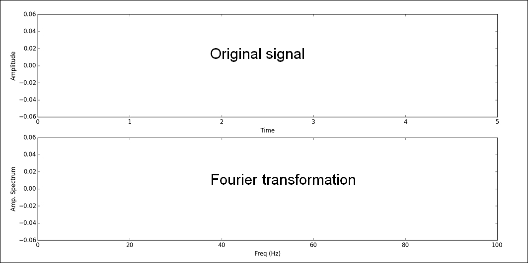
The upper plot area shows the original functions (signal), and the lower plot shows the Fourier transformation. Please type the following code into your IPython command prompt or save it to a .py file and load it to the prompt:
#### The Plotting Functions ####import matplotlib.pyplot as plt
import numpy as np
def show(ori_func, ft, sampling_period = 5):
    n = len(ori_func)
    interval = sampling_period / n
    plt.subplot(2, 1, 1)
    plt.plot(np.arange(0, sampling_period, interval), ori_func, 'black')
    plt.xlabel('Time'), plt.ylabel('Amplitude')
    plt.subplot(2,1,2)
    frequency = np.arange(n / 2) / (n * interval)
    nfft = abs(ft[range(int(n / 2))] / n )
    plt.plot(frequency, nfft, 'red')
    plt.xlabel('Freq (Hz)'), plt.ylabel('Amp. Spectrum')
    plt.show()
This is a display function called show(), which has two input parameters: the first one is the original signal function (ori_func) and the second one is its Fourier transform (ft). This method will use the matplotlib.pyplot module to create two line charts: the original signal at the top with black lines, where the x axis represents the time intervals (we set the default signal sampling period to be five seconds for our all examples) and the y axis represents the amplitude of the signal. The lower part of the chart is its Fourier transform with a red line, where the x axis represents the frequency and the y axis represents the amplitude spectrum.
In the next section, we will simply go through different types of signal waves and use the numpy.fft module to compute the Fourier transform. Then we call the show() function to provide a visual comparison between them.