SciPy is a well-known Python library focusing on scientific computing (it contains modules for optimization, linear algebra, integration, interpolation, and special functions such as FFT, signal, and image processing). It builds on the NumPy Array object, and NumPy is part of the whole SciPy stack (remember that we introduced the Scientific Python family in Chapter 1, An Introduction to NumPy). However, the SciPy module contains various topics that we can't cover in just one section. Let's look at an example of image processing (noise removal) to help you get some idea of what SciPy can do:

In [1]: from scipy.misc import imread, imsave, ascent 
In [2]: import matplotlib.pyplot as plt 
In [3]: image_data = ascent() 

First, we import three functions from SciPy's miscellaneous routines: imread, imsave, and ascent. In the following example, we use the built-in image ascent, which is a 512 by 512 greyscale image. Of course, you may use your own image; simply call imread('your_image_name') and it will load as an ndarray.

The pyplot result from the matplotlib module we imported here is just for displaying the image; we did this in Chapter 6, Fourier Analysis in NumPy. Here is the built-in image ascent:

Now, we can add some noise to the image and use the pyplot module to show the noised image:

In [4]: import numpy as np 
In [5]:noise_img = image_data +  image_data.std() * np.random.random(image_data.shape) 
In [6]: imsave('noise_img.png', noise_img) 
In [7]: plt.imshow(noise_img) 
Out[7]: <matplotlib.image.AxesImage at 0x20066572898> 
In [8]: plt.show() 

In this code snippet, we import numpy to generate some random noise based on the image shape. Then, we save the noised image to noise_img.png. The noised image looks like this:

Next, we are going to use the multidimensional image-processing module in SciPy, scipy.ndimage, to apply filters to the noised image in order to smooth it. The ndimage module provides various filters; for a detailed list, refer to http://docs.scipy.org/doc/scipy/reference/ndimage.html, but in the following example, we will just use the Gaussian and Uniform filters:

In [9]: from scipy import ndimage 
In [10]: gaussian_denoised = ndimage.gaussian_filter(noise_img, 3) 
In [11]: imsave('gaussian_denoised.png', gaussian_denoised ) 
In [12]: plt.imshow(gaussian_denoised) 
Out[12]: <matplotlib.image.AxesImage at 0x2006ba54860> 
In [13]: plt.show() 
In [14]: uniform_denoised = ndimage.uniform_filter(noise_img) 
In [15]: imsave('uniform_denoised.png', uniform_denoised) 
In [16]: plt.imshow(gaussian_denoised) 
Out[17]: <matplotlib.image.AxesImage at 0x2006ba80320> 
In [18]: plt.show() 

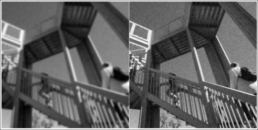
First, we import ndimage from SciPy, apply the Gaussian filter on noise_image, set the sigma (the standard deviation for the Gaussian kernel) to 3, and save it to gaussian_denoised.png. Look at the the left-hand side of the preceding image. In general, the larger the sigma, the smoother the image will be, which means a loss of detail. The second filter we applied is the Uniform filter and took all the default values for the parameters, which results in the right-hand part of the previous image. Though the uniform filter retains more details from the raw image, the image still contains noise.

The previous example was a simple image-processing example using SciPy. However, SciPy can do more than image processing, it can also perform many types of analytical/scientific computation. For details, refer to Learning SciPy for Numerical and Scientific Computing, Second Edition, Packt Publishing.