Scikit is short for SciPy Toolkits, which are add-on packages for SciPy. It provides a wide range of analytics modules and scikit-learn is one of them; this is by far the most comprehensive machine learning module for Python. scikit-learn provides a simple and efficient way to perform data mining and data analysis, and it has a very active user community.

You can download and install scikit-learn from its official website at http://scikit-learn.org/stable/. If you are using a Python scientific distribution, such as Anaconda, it is included here as well.

Now, it's time for some machine learning using scikit-learn. One of the advantages of scikit-learn is that it provides some sample datasets (demo datasets) for practice. Let's load the diabetes dataset first.

In [1]: from sklearn.datasets import load_diabetes 
In [2]: diabetes = load_diabetes() 
In [3]: diabetes.data 
Out[3]: 
array([[ 0.03807591,  0.05068012,  0.06169621, ..., -0.00259226, 
         0.01990842, -0.01764613], 
       [-0.00188202, -0.04464164, -0.05147406, ..., -0.03949338, 
        -0.06832974, -0.09220405], 
       [ 0.08529891,  0.05068012,  0.04445121, ..., -0.00259226, 
         0.00286377, -0.02593034], 
       ..., 
       [ 0.04170844,  0.05068012, -0.01590626, ..., -0.01107952, 
        -0.04687948,  0.01549073], 
       [-0.04547248, -0.04464164,  0.03906215, ...,  0.02655962, 
         0.04452837, -0.02593034], 
       [-0.04547248, -0.04464164, -0.0730303 , ..., -0.03949338, 
        -0.00421986,  0.00306441]]) 
In [4]: diabetes.data.shape 
Out[4]: (442, 10) 

We loaded a sample dataset called diabetes from sklearn.datasets; it contains 442 observations, 10 dimensions, and ranges from -2 to 2. The Toy dataset also provides labeled data for supervised learning (if you are not familiar with machine learning, try to think of the labelled data as categories). In our example, labeled data from the diabetes dataset can be called from diabetes.target, and it has a range from 25 to 346.

Remember how we performed linear regression in Chapter 5 , Linear Algebra in Numpy? We're going to perform it one more time using scikit-learn instead. Again, I recommend that, when you're developing a script to help you in your research or analytics, use NumPy ndarray as your general data format; however, for computation, using scipy, scikit-learn, or other scientific modules would be more preferable. One advantage of machine learning is model evaluation (where you train and test the result). Using this, we will split our data into two datasets: training datasets and test datasets, and then pass the two datasets for the purpose of linear regression:

In [5]: from sklearn.cross_validation import train_test_split 
In [6]: X_train, X_test, y_train, y_test  = 
        train_test_split(diabetes.data, 
diabetes.target, 
random_state = 50) 

In the preceding example, we split up the diabetes dataset into training and test datasets (for both the data and its categories) using the train_test_split() function. The first two parameters are arrays that we want to split; the random_state parameter is optional, which means that a pseudo random number generator state is used for random sampling. The default split ratio is 0.25, which means that 75% of the data is split into the training set and 25% is split into the test set. You can try to print out the training/test datasets we just created to take a look at its distribution (in the preceding code example, X_train represents the training dataset for the diabetes data, X_test represents the diabetes test data, y_train represents the categorized diabetes training data, and y_test represents the categorized diabetes test data).

Next, we are going to fit our datasets into a linear regression model:

In [7]: from sklearn.linear_model import LinearRegression 
In [8]: lr = LinearRegression() 
In [9]: lr.fit(X_train, y_train) 
Out[9]: LinearRegression(copy_X = True, fit_intercept = True, 
     Normalize = False) 
In [10]: lr.coef_ 
Out[10]: 
array([  80.73490856, -195.84197988,  474.68083473,  371.06688824, 
       -952.26675602,  611.63783483,  174.40777144,  159.78382579, 
        832.01569658,   12.04749505]) 

First, we created a LinearRegression object from sklearn.linear_model and used the fit() function to fit the X_train and y_train datasets. We can check the estimated coefficients for the linear regression by calling its coef_ attribute. Furthermore, we can use the fitted linear regression for prediction. Take a look at the following example:

In [11]: lr.predict(X_test)[:10] 
Out[11]: 
array([  71.96974998,   82.55916305,  265.71560021,   79.37396336, 
         72.48674613,   47.01580194,  149.11263906,  185.36563936, 
         94.88688296,  132.08984366]) 

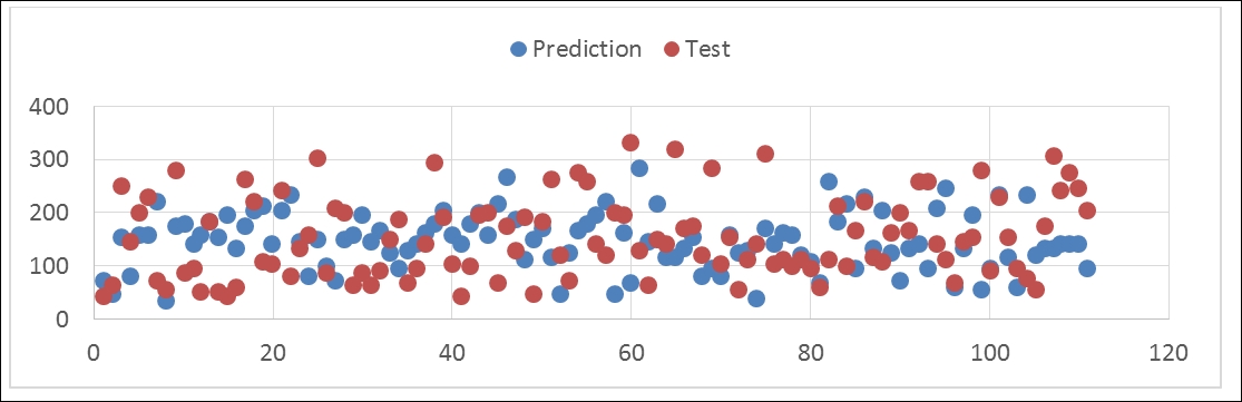
The predict() function is used to predict the test dataset based on the linear regression we fit with the training datasets; in the preceding example, we printed out the first 10 predicted values. Here is the plot of the predicted and test value of y:

In [12]: lr.score(X_test, y_test) 
Out[12]: 0.48699089712593369 

Then, we can check the determination R-square of the prediction using the score() function.

This is pretty much the standard fitting and predicting process in scikit-learn, and it's pretty intuitive and easy to use. Of course, besides regression, there are many analytics that scikit-learn can carry out such as classification, clustering, and modeling. Hope this section helps you in your scripts.