There are many ways to define the DFT; however, in a NumPy implementation, the DFT is defined as the following equation:

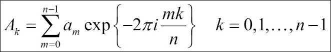
A _k represents the discrete Fourier transform and a_m represents the original function. The transformation from a_m->A_k is a translation from the configuration space to the frequency space. Let's calculate this equation manually to get a better understanding of the transformation process. We will use a random signal with 500 values:

In [25]: x = np.random.random(500) 
In [26]: n = len(x) 
In [27]: m = np.arange(n) 
In [28]: k = m.reshape((n, 1)) 
In [29]: M = np.exp(-2j * np.pi * k * m / n) 
In [30]: y = np.dot(M, x) 

In this code block, x is our simulated random signal, which contain 500 values and corresponds to a_m in the equation. Based on the size of x, we calculate the sum product of:

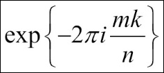
We then save it to M. The final step is to use the matrix multiplication between M and x to generate DFT and save it to y.

Let's verify our result by comparing it with the built-in numpy.fft:

In [31]: np.allclose(y, np.fft.fft(x)) 
Out[31]: True 

As we expected, the manually computed DFT is identical to the NumPy built-in module. Of course, numpy.fft is just like any other built-in modules in NumPy-it's been optimized and the FFT algorithm has been applied. Let's compare the performance between our manual DFT and numpy.fft:

In [32]: %timeit np.dot(np.exp(-2j * np.pi * np.arange(n).reshape((n, 1)) * np.arange(n) / n), x) 
10 loops, best of 3: 18.5 ms per loop 
In [33]: %timeit np.fft.fft(x) 
100000 loops, best of 3: 10.9 µs per loop 

First, we put this equation implementation code on one line in order to measure the execution time. We can see a huge performance difference between them. Underneath the hood, NumPy uses the FFTPACK library to perform the Fourier transform, which is a very stable library both in performance and accuracy.

Next, we are going to compute the inverse DFT. The iDFT maps the frequency series back to the original time series, which is defined in the following equation:

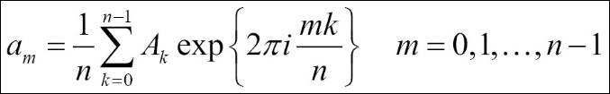
We can see the inverse equation differs from the DFT equation by the sign of the exponential argument and the normalization by 1/n. Let's do the manual calculation again. We can re-use the m, k, and n variables from the previous code and just re-compute M due to the sign change of the exponential argument:

In [34]: M2 = np.exp(2j * np.pi * k * m / n) 
In [35]: x2 = np.dot(y, M2) / n 

Again, let's verify the computed inverse DFT result x2 with our original random signal x. The two ndarray should be identical:

In [36]: np.allclose(x, x2) 
Out[36]: True 

Of course, the numpy.fft module also support inverse DFT-simply call numpy.fft.ifft() to perform the computation, as you can see in the following example:

In [37]: np.allclose(x, np.fft.ifft(y)) 
Out[37]: True 

You may notice that, in the previous examples, we always use a one-dimensional array as our input signals. Does that mean that numpy.fft only handles one-dimensional data? Of course not; numpy.fft can also process two- or multi-dimensional data. Before we get to this part, we'd like to talk about the order of returned FFT arrays and a shift method in numpy.fft.

Let's create a simple signal array with 10 random integers, and compute its Fourier transform:

In [38]: a = np.random.randint(10, size = 10) 
In [39]: a 
Out[39]: array([7, 4, 9, 9, 6, 9, 2, 6, 8, 3]) 
In [40]: a.mean() 
Out[40]: 6.2999999999999998 
In [41]: A = np.fft.fft(a) 
In [42]: A 
Out[42]: 
array([ 63.00000000 +0.00000000e+00j,   
        -2.19098301 -6.74315233e+00j, 
        -5.25328890 +4.02874005e+00j, 
        -3.30901699 -2.40414157e+00j, 
        13.75328890 -1.38757276e-01j,    
      1.00000000 -2.44249065e-15j, 
        13.75328890 +1.38757276e-01j, 
     -3.30901699 +2.40414157e+00j, 
        -5.25328890 -4.02874005e+00j, 
     -2.19098301 +6.74315233e+00j]) 
In [43]: A[0] / 10 
Out[43]: (6.2999999999999998+0j) 
In [44]: A[int(10 / 2)] 
Out[44]: (1-2.4424906541753444e-15j) 

In this example, a is our original random signal and A is a's Fourier transform. When we call numpy.fft.fft(a), the resulting ndarray follows the "standard" order in which the first value A[0] contains the zero-frequency term (the mean of the signal). When we do the normalization, which is dividing it by the length of the original signal array (A[0] / 10), we get the same value as when we calculated the mean of the signal array (a.mean()).

Then A[1:n/2] contains the positive-frequency terms and A[n/2 + 1: n] contains the negative-frequency terms. When the inputs are even numbers as in our example, A[n/2] represents both positive and negative. If you want to shift the zero-frequency component to the center of the spectrum, we can use the numpy.fft.fftshift() routine. See the following example:

In [45]: np.fft.fftshift(A) 
Out[45]: 
array([  1.00000000 -2.44249065e-15j,   
     13.75328890 +1.38757276e-01j, 
        -3.30901699 +2.40414157e+00j, 
        -5.25328890 -4.02874005e+00j, 
        -2.19098301 +6.74315233e+00j, 
        63.00000000 +0.00000000e+00j, 
        -2.19098301 -6.74315233e+00j, 
     -5.25328890 +4.02874005e+00j, 
        -3.30901699 -2.40414157e+00j,   
     13.75328890 -1.38757276e-01j]) 

From this example, you can see that numpy.fft.fftshift() swaps half-spaces in the array, so the zero-frequency components are shifted to the middle. numpy.fft.ifftshift is the inverse function, shifting the order back to "standard".

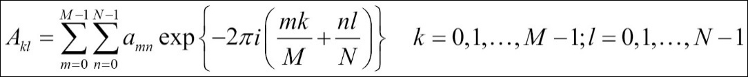
Now, we are going to talk multi-dimensional DFT; let's start with two dimensions. You may see that the following equation is very similar to a one-dimensional DFT, and the second dimension is extended in the obvious way. The idea for multi-dimensional DFT is the same, and so does the inverses in higher dimensions. You may also try to modify the previous codes to calculate the one-dimensional DFT to two or multi-dimensional DFT to better understand the processes. But now we are simply going to demonstrate how to use numpy.fft for two-dimensional and multi-dimensional Fourier transforms:

In [46]: x = np.random.random(24) 
In [47]: x.shape = 2,12 
In [48]: y2 = np.fft.fft2(x) 
In [49]: x.shape = 1,2,12 
In [50]: y3 = np.fft.fftn(x, axes = (1, 2)) 

From these examples, you can see that we call numpy.fft.fft2() for a two-dimensional Fourier transform, and numpy.fft.fftn() for multi-dimensional. The axes parameter is optional; it indicates the axes over which to compute the FFT. For two-dimensional, if the axes are not specified, it uses the last two axes; while for multi-dimensional, the module uses all the axes. In the previous example, we applied the last two axes only, so the Fourier transform result will be identical to the two-dimensional one. Let's check it out:

In [51]: np.allclose(y2, y3) 
Out[51]: True