
Optimum Bidding of Renewable Energy System Owners in Electricity Markets
Ting Dai, Siemens, Greater Minneapolis-St. Paul, MI, United States
Abstract
The main challenge faced by the renewable energy system owners in the electricity market comes from the uncertainty of the renewable energy productions. To help them survive in the competitive market, this chapter introduced the stochastic programming to model the uncertainties and build bidding strategies for the renewable energy owners. Two types of the renewable energy owners—price-takers and price-makers are considered in this chapter and different models are proposed accordingly. The conditional value at risk is used to compute the risks associated with the bidding strategies. The case studies using real-world data are presented to show the effectiveness of the proposed models.
Keywords
Renewable energy; electricity market; bidding strategies; stochastic programming
4.1 Renewable Energy System Owners in Electricity Markets
4.1.1 Electricity Market Overview
The electric power industry has evolved from a regulated operational structure to a competitive one in many countries around the world. In the United States, the Federal Energy Regulatory Commission established the foundation for developing competitive bulk electricity markets by enacting order 888 and 889 in 1996 to ensure nondiscriminatory open access to transmission services. Since then, the electricity industry has encountered numerous reconstruction activities, including increasing the number of market participants and the establishment of market operators as managers of a fair and secure market environment. Up to now, about two-thirds of the US electricity load is operated in the electricity markets.
Based on the type of production to be traded, the electricity market can be categorized into the energy market, ancillary services market, financial transmission rights (FTR) market, and capacity market.
1. Energy market (also known as “the pool-based market”). Energy is bought and sold in the energy market through a two-settlement process: Day-ahead (DA) market and real-time (RT) market (also known as the balancing market). The DA market clears energy transactions each hour of the next operating day, whereas RT market transactions are performed just minutes before actual power deliveries. Energy is bought and sold in the RT market at RT spot prices to make up imbalances when system conditions change from the DA market. In some European countries, the energy market also includes an adjustment market which is similar to the DA market but is cleared closer to power delivery. The adjustment market is not discussed in this chapter.
2. Ancillary services market. In addition to the energy market, the ancillary services market ensures the reliability of the power system. Various types of ancillary services exist in the market today, such as regulation, contingency, and reserves. Other ancillary services, such as voltage control and black start services do not typically have auction-based markets.
3. FTR market. In the FTR markets, forward auctions are held to allow market participants to submit their bids for purchase and sale of transmission rights. The transmission rights holders can obtain revenues or be charged penalties based on the locational differences in hourly energy prices.
4. Capacity market. The capacity market ensures long-term grid reliability by procuring the appropriate power capacity that is needed to meet growth predictions for future demand. This market creates long-term price signals and attracts promising bidders to invest in different resource supplies.
The scope of this chapter includes only the US short-term energy markets which are DA market and RT market.
4.1.1.1 Electricity Market Participants and Operators
The participants in an electricity market can be divided into three categories
1. Consumers. They are end users who buy energy or services (such as reserves) from the electricity market. A consumer can submit consumption bids to the electricity market with the goal of minimizing the cost of purchasing energy or services.
2. Retailers. They submit bids to purchase energy or services from the electricity market and sell them back to the consumers who don’t participate directly in the electricity market.
3. Energy Owners. They provide energy or services by submitting offers in the electricity market. Their intention is to maximize their total profits from selling energy or services.
With so many participants in the electricity market, a neutral entity is required to establish sound market rules to guarantee the functioning of the economy and the processing of secure transactions. In the United States, independent system operators (ISOs) or regional transmission organizations (RTOs) are used to fulfill this role. The ISOs or RTOs administer transmission tariffs, maintain system security levels, coordinate and schedule maintenance, and play an important role in coordinating long-term planning. In the electricity market, the ISOs/RTOs play an important role as independent, unaffiliated market operators providing unbiased, open access to all market participants. The ISOs/RTOs also forecast electricity demand, schedule adequate reserve, run market clearing models, and send price signals to all of the market participants.
4.1.1.2 Time Frame of the Short-Term Electricity Market
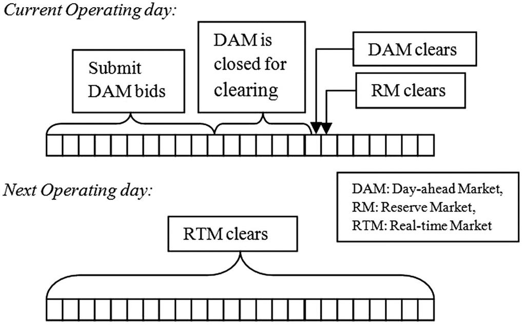
The time framework for the short-term electricity market is shown in Fig. 4.1. The DA market, as its name implies, refers to the market that operates 24 h prior to the RT market. It is used for scheduling the power production for the next day. The reserve market operates almost at the same time as the DA market. In most US markets, the DA market and reserve market are cooptimized by using a single clearing process, as determined by the ISOs/RTOs, from which the energy and reserve transactions are determined during each hour of the next operating day. Once the markets are cleared, the locational marginal prices (LMP), the reserve clearing prices, and the cleared energy volume of each participant are settled. The RT market is carried out just minutes before the actual power delivery by energy owners to ensure a RT balance between generation and demand. This is done by offsetting the differences between the RT operation and the corresponding energy program settled in the DA market. RT prices are calculated for the RT market based on the operating conditions.
4.1.1.3 Energy Owners in the Electricity Market
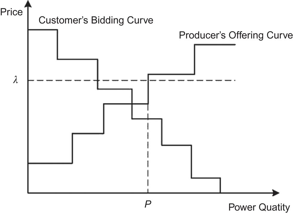
In the short-term electricity market, the energy owners submit nondecreasing stepwise offering curves and the customers submit nonincreasing stepwise bidding curves indicating their willingness to sell and buy certain amounts of energy or reserve at certain prices, respectively. An illustration of an energy owner’s offering curve and a customer’s bidding curve is shown in Fig. 4.2. The ISOs/RTOs aggregate all of the bidding and offering curves, and determine the market clearing prices and power quantity committed from each energy owner and customer. As shown in Fig. 4.2, if the market clearing price is λ, the committed power of the energy owner is P. Failing to fulfill their commitments brings penalties to the energy owners. The RT penalty mechanisms are not the same in the electricity markets of different countries. For example, in most European countries, two RT prices are determined separately in two different situations: a positive RT price for positive energy deviation (higher production or lower consumption than scheduled) and a negative RT price for negative energy deviation (lower production or higher consumption than scheduled).
4.1.2 Importance of Integrating Renewables into the Electricity Market
Before entering the electricity market, wind power is sold through long-term power purchase agreements (PPAs) which require the purchasers to buy all of the wind energy generated at a fixed price. However, after topping out at nearly $70/MW h for PPAs executed in 2009, the national average price of PPAs has shown a continuously declining trend [1]. In 2014, wind PPA prices fell to the lowest point at $23.5/MW h, which is almost competitive with wholesale prices in the electricity market. Also, since the availability of PPA contracts for wind remain in short supply, wind power energy owners can no longer obtain stable revenues by selling their power through PPAs. Studies show that wind energy integration costs are almost always below $12/MW h and often below $5/MW h—for wind power capacity penetrations of up to or even exceeding 40% of the peak load of the system in which the wind power is delivered. System operators continue to implement a range of methods to accommodate increased wind energy penetrations, including: centralized wind forecasting, treating wind as dispatchable, shorter scheduling intervals, and balancing areas consolidation and coordination.
Today, around 23% of the wind power capacity in the United States is sold either through short-term contracts or directly into the electricity market. This percentage is expected to increase further according to the authors of the report [1]. They mentioned another important factor. The recent completion of transmission lines in Texas provides market access to a significant amount of newly installed wind capacity. As a consequence, wind energy owners are becoming more and more interested in trading their power in the electricity market instead of locking their revenues in the PPAs.
4.1.3 Current Market Rules for Renewable Energy System Owners in North America
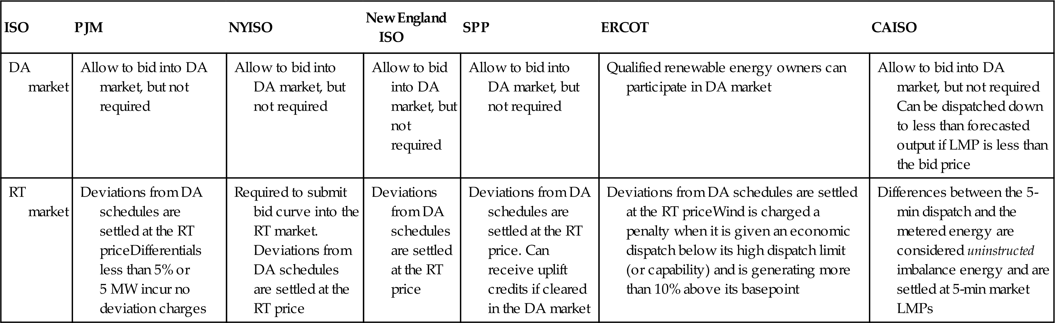
Nowadays, wind and solar energy owners are permitted to participate in DA and RT market in North America but are not required to do so. For example, New England ISO has allowed renewable system owners to submit energy bid curve or self-schedule into the DA market (can include negative price bids). The proposal to require wind to submit bid curves into the DA market is under consideration. In most of the RT markets, renewable energy owners are not fully penalized for their deviation from DA schedule. Pennsylvanian–New-Jersey–Maryland interconnection (PJM) charges no penalty for deviation power less than 5% or 5 MW; Electric Reliability Council of Texas (ERCOT) charges wind a penalty when it is given an economic dispatch below its high dispatch limit (or capability) and is generating more than 10% above its basepoint. However, treating renewable energy owners the same way as the conventional power owners is a trend for the electricity markets. Table 4.1 provides the summary of the rules for integrating renewable energy in six North America electricity DA and RT markets: PJM, New York ISO (NYISO), New England ISO, southwest power pool (SPP), ERCOT, and California (CAISO). For more detailed information, please refer to Ref. [2].
Table 4.1
Rules for Renewable Energy Owner to Participate in DA and RT Markets
| ISO | PJM | NYISO | New England ISO | SPP | ERCOT | CAISO |
| DA market | Allow to bid into DA market, but not required | Allow to bid into DA market, but not required | Allow to bid into DA market, but not required | Allow to bid into DA market, but not required | Qualified renewable energy owners can participate in DA market | Allow to bid into DA market, but not required Can be dispatched down to less than forecasted output if LMP is less than the bid price |
| RT market | Deviations from DA schedules are settled at the RT priceDifferentials less than 5% or 5 MW incur no deviation charges | Required to submit bid curve into the RT market. Deviations from DA schedules are settled at the RT price | Deviations from DA schedules are settled at the RT price | Deviations from DA schedules are settled at the RT price. Can receive uplift credits if cleared in the DA market | Deviations from DA schedules are settled at the RT priceWind is charged a penalty when it is given an economic dispatch below its high dispatch limit (or capability) and is generating more than 10% above its basepoint | Differences between the 5-min dispatch and the metered energy are considered uninstructed imbalance energy and are settled at 5-min market LMPs |
In this chapter, the market bidding rules applied to conventional energy owners are assumed to be applied to the renewable energy owners. The renewable energy owners can submit multisegment bidding curves into the both DA and RT market. The deviation from DA schedule will be settled in RT price: if the actual production is less than the DA scheduled, the renewable energy owners will have to buy the deviated power at the RT price; otherwise, the renewable energy owners can bid the extra power into the RT market and get paid for the accepted power at the RT prices.
Thus, the profit of the renewable energy owner ![]() can be expressed as:
can be expressed as:
(4.1)
where ![]() and
and ![]() are DA and RT market clearing prices.
are DA and RT market clearing prices. ![]() and
and ![]() are power scheduled in DA and RT.
are power scheduled in DA and RT.
As can be seen from Eq. (4.1), ![]() and
and ![]() are both uncertain variables.
are both uncertain variables. ![]() and
and ![]() are variables determined by the renewable energy owners but are also constrained by the actual power production which is also uncertain. In order to obtain the maximum revenue of the renewable energy owners, optimization models need to take consideration of these uncertain variables.
are variables determined by the renewable energy owners but are also constrained by the actual power production which is also uncertain. In order to obtain the maximum revenue of the renewable energy owners, optimization models need to take consideration of these uncertain variables.
4.2 Price-Taker Models—MultiStage Stochastic Programming Approach
4.2.1 MultiStage Stochastic Programming Approach
Stochastic programming is an approach for modeling optimization problems that involves uncertainties. In the short-term electricity market, decision makers have to make optimal decisions throughout a decision horizon involving several stages. For example, DA market decisions are first-stage decisions which are made before knowing the market clearing prices in the DA and RT markets. RT market decisions, on the other hand, are made after the clearing of the DA market but before knowing the market clearing prices in the RT market, which constitutes second-stage decisions. Thus, a two-stage stochastic programming model would be an appropriate tool for energy owners trading in both DA and RT markets.
In stochastic programming, the stochastic process, such as electricity market prices and wind power production, can be represented using continuous or discrete random variables. In a best case scenario, stochastic programming problems with continuous random variables can only be solved in small or illustrative instances [3]. For this reason, scenario representation of random variables becomes indispensable in solving stochastic problems. The set of values used to model a random variable is usually arranged in a so-called “scenario tree,” as illustrated in Fig. 4.3. A scenario tree comprises a set of nodes and arcs. The node in the first-stage is called the root node. The nodes in the last stage are called leaves. A scenario is a path from the root to the leaf. A stage is a moment in the time line when the decisions are taken.

4.2.2 Scenario Generation and Reduction Method
Different techniques have been proposed in the literature to generate scenarios and build scenario trees. An easy way to generate a scenario for market prices is the sampling method, as proposed in Ref. [4]. Høyland and Wallace [5] proposed a moment matching method to generate a limited number of scenarios which satisfied certain properties. Pflug [6] described an optimal discretization method to find the reduced scenario set of the initial one that minimizes an error based on an objective function.
Given that the computational burden of a stochastic programming problem increases rapidly with the number of scenarios, scenario reduction becomes necessary. The scenario reduction techniques for two-stage stochastic programming were presented in Refs. [7,8]. The reduced number of scenarios that best retains the essential features of the original scenario set is chosen according to a probability distance.
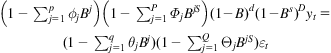
In this chapter, a procedure combining a path-based method and a scenario reduction technique is used to generate multistage scenario trees [9]. A seasonal autoregressive integrated moving average (ARIMA) model [10] is used to generate a large number of scenarios for uncertainties in the market. The general expression of seasonal ARIMA model can be expressed as follows:
(4.2)
 (4.2)
(4.2)
with ![]() autoregressive parameter
autoregressive parameter ![]() ,
, ![]() moving average parameter
moving average parameter ![]() , a seasonal component of
, a seasonal component of ![]() autoregressive parameter
autoregressive parameter ![]() ,
, ![]() moving average parameter
moving average parameter ![]() , and where
, and where ![]() and
and ![]() are the actual value and error at time t, respectively.
are the actual value and error at time t, respectively. ![]() is the backshift operator, that is,
is the backshift operator, that is, ![]() .
.
As ![]() is the forecast error which a random variable following normal distribution, a large number of scenarios can be generated by generating random value for
is the forecast error which a random variable following normal distribution, a large number of scenarios can be generated by generating random value for ![]() . Then, a fast-forward scenario-reduction algorithm [9] was used to obtain a reduced scenario set with a sufficiently small number of scenarios from an iterative process. In each iteration, the scenario that minimized the Kantorovich distance between the reduced set and the original set is chosen from the set of unselected scenarios and included in the reduced set. The algorithm stops if either the required number of scenarios or a certain Kantorovich distance is attained. Fig. 4.4 shows an example of generating 10 DA LMP scenarios for each during one week by using PJM data [11].
. Then, a fast-forward scenario-reduction algorithm [9] was used to obtain a reduced scenario set with a sufficiently small number of scenarios from an iterative process. In each iteration, the scenario that minimized the Kantorovich distance between the reduced set and the original set is chosen from the set of unselected scenarios and included in the reduced set. The algorithm stops if either the required number of scenarios or a certain Kantorovich distance is attained. Fig. 4.4 shows an example of generating 10 DA LMP scenarios for each during one week by using PJM data [11].

4.2.3 Risk Management
Despite the numerous advantages of using stochastic programming to model the uncertainties associated with wind power trading, it only shows that the decision makers expect profits and neglect the probabilities of negative profits or losses. Thus, risk management constitutes an important part of the stochastic programming and helps the decision makers avoid undesirable outcomes.
Different types of risk management models have been reported and analyzed, such as the variance, the shortfall probability, the VaR [12], and the conditional value at risk (CVaR) [13] models.
For a given ![]() , VaRα is a measure computed as the maximum profit value such that the probability of the profit being lower than or equal to this value is lower than or equal to 1−α.
, VaRα is a measure computed as the maximum profit value such that the probability of the profit being lower than or equal to this value is lower than or equal to 1−α.
(4.3.1)
where p and B represent the probability and expected value of the profit, respectively, x is the decision variable of the maximization problem (4.3.1–4.3.5).
For a given ![]() , the CVaRα represents the expected value not surpassing VaRα.
, the CVaRα represents the expected value not surpassing VaRα.
(4.3.2)
A discrete formulation of CVaRα is the following:
(4.3.3)
Subject to
(4.3.4)
(4.3.5)
where ![]() and
and ![]() represent the probability and expected profit of scenario ω, respectively,
represent the probability and expected profit of scenario ω, respectively, ![]() is an auxillary variable used to compute CVaR, and
is an auxillary variable used to compute CVaR, and ![]() an auxillary variable used to compute CVaR in scenario ω.
an auxillary variable used to compute CVaR in scenario ω.
There is an additional difficulty in using VaR for stochastic problems in that it requires the use of binary variables for its modeling. Instead, the computation of CVaR does not require the use of binary variables; and it can be simply modeled by using linear constraints. The CVaR has been successfully implemented in various models considering uncertainties. Especially for wind energy owners, CVaR can help the decision makers to model the tradeoff between profit and risk.
4.2.4 Bidding Strategy Models for Price-Taker Renewable Energy Owner
In this section, we will model the bidding strategy for the price-taker renewable energy owner using multistage stochastic programming. The mathematical formulation will be presented and a simple example will be shown.
4.2.4.1 Basic Mathematical Formation for the Price-Taker Renewable Energy Owner
The basic mathematical formulation for the price-taker renewable energy owner in DA and RT market are expressed in the following mathematical problem (4.4):
(4.4.1)
 (4.4.1)
Subject to
(4.4.2)
(4.4.3)
(4.4.4)
(4.4.5)
(4.4.6)
(4.4.7)
(4.4.8)
(4.4.9)
(4.4.10)
where ![]() ,
, ![]() ,
, ![]() ,
,![]() ,
, ![]() , and
, and ![]() are the decision variables.
are the decision variables. ![]() represents the power offered by the renewable energy owner in the DA market at time period t.
represents the power offered by the renewable energy owner in the DA market at time period t. ![]() ,
, ![]() , and
, and ![]() represent the positive deviation, negative deviation, and total deviation of the renewable energy owner in the RT market at time period t.
represent the positive deviation, negative deviation, and total deviation of the renewable energy owner in the RT market at time period t.
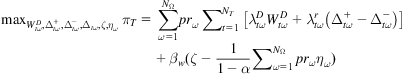
The objective function comprises two terms: (1) The expected profit of the renewable energy owner, which equals the revenue from the DA market plus the revenue from positive energy deviations in the RT market minus the cost for negative energy deviations in the RT market; and (2) the CVaR multiplied by a weighting factor βW, which controls the degree of risk aversion of the renewable energy owner.
In this model, the first-stage decision variable is the hourly bid of the energy volume ![]() of the renewable energy owner, whereas the second-stage variables are the RT energy deviations
of the renewable energy owner, whereas the second-stage variables are the RT energy deviations ![]() and
and ![]() of the renewable energy owner. Constraint (4.4.2) limits the amount of wind energy that can be traded in the DA market. Constraints (4.4.3)–(4.4.6) determine the total positive and negative energy deviations incurred by the wind energy owner per period and scenario. Constraint (4.4.7) constitutes the nonanticipativity conditions related to the decisions made in the first-stage. Constraint (4.4.8) enforces a nondecreasing offer curve. Constraints (4.4.9) and (4.4.10) are used to compute CVaR.
of the renewable energy owner. Constraint (4.4.2) limits the amount of wind energy that can be traded in the DA market. Constraints (4.4.3)–(4.4.6) determine the total positive and negative energy deviations incurred by the wind energy owner per period and scenario. Constraint (4.4.7) constitutes the nonanticipativity conditions related to the decisions made in the first-stage. Constraint (4.4.8) enforces a nondecreasing offer curve. Constraints (4.4.9) and (4.4.10) are used to compute CVaR.
4.2.4.2 Examples
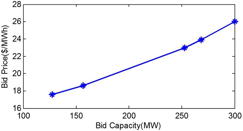
In this section, we will present the example to demonstrate the effectiveness of the proposed model in the previous section. The historical data speed and market prices are obtained from PJM website [11]. The maximum wind generating capacity is set to be 300 MW. The ARIMA model is used to generate 5000 scenarios for wind power production, DA, respectively. Then, the scenario reduction method is applied to reduce the number of scenarios for each uncertainty to 5. Table 4.2 shows the information of these scenarios. The risk control parameter is set to be 0.2.
Table 4.2
| Scenario # | Wind Power Production (MW) | Probability | DA LMP ($/MW h) | Probability |
| 1 | 109.52 | 0.302 | 17.55 | 0.251 |
| 2 | 150.20 | 0.2049 | 17.58 | 0.271 |
| 3 | 205.53 | 0.105 | 22.97 | 0.178 |
| 4 | 251.98 | 0.187 | 23.90 | 0.160 |
| 5 | 289.61 | 0.201 | 26.03 | 0.139 |

By solving problem (4.4), the bidding strategy capacity into DA market for each scenario is ![]() ,
, ![]() ,
,![]() ,
,![]() ,
,![]() . Using these solved bidding capacities and their corresponding DA LMP, the readers can build the nondecreasing bidding curve shown in Fig. 4.5.
. Using these solved bidding capacities and their corresponding DA LMP, the readers can build the nondecreasing bidding curve shown in Fig. 4.5.
The risk management control parameter can be used to control the risk associated with uncertainties. As we increase βW, the value of CVaR increases; but the expected profit decreases as shown in Figs. 4.6 and 4.7. This is as expected, the energy owner increases βW in order to reduce the trading risks, thus, the cost associated with risks increase and the expected profit decreases.


4.2.5 Mitigating the Trading Risk by Purchasing Additional Power from Conventional Energy Owner
4.2.5.1 Introduction
To mitigate the trading risk associated with renewable energy trading, many approaches have been discussed and applied, such as combining renewable energy units with energy storage system, signing bilateral contract, and others. In this chapter, we will introduce the approach to mitigate the risk for bidding in the electricity market by buying additional amount of power from conventional energy owner and use it as “reserve” to hedge against the RT market penalties.
In Ref. [14], the authors introduced a bilateral reserve settlement mechanism between renewable energy owners and conventional energy owners. The authors proposed several assumptions: (1) The bilateral reserve settlement introduced can be mixed with the system-wide reserve to provide standby power to cover the intermittency and uncertainty of renewable energy sources. The bilateral reserve is provided by conventional energy owners and consumed by renewable energy owners. (2) The bilateral reserve settlement among renewable and conventional energy owners can be seen as a new trading mechanism for a new type of reserve, adding to the existing system-wide reserve. The bilateral reserve settlement price and volumes of specific providers are cleared among the renewable and conventional energy owners who provide this new type of reserve. This new bilateral trading mechanism does not change current implementation of the system-wide reserve, regulation, and other auxiliary services for mitigating other uncertainties, for example, large load uncertainties, in the system.
Both renewable and conventional energy owners try to compete with other energy owners and maximize their profit in the market. The bilateral reserve price and power amount settled between these two types of energy owners can be solved using game theory. The optimal bidding strategy of both energy owners can be modeled using stochastic programming introduced in the previous section.
4.2.5.2 Auction Game and Nash Equilibrium
This section gives an introduction of game theory, Nash Equilibrium, and the application settle the bilateral reserve price and power amount between conventional and renewable energy owners.
A game is a “formal representation of a situation in which a number of individuals interact in a setting of strategic independence [15].” There are four elements in a game: (1) The players, (2) the rules of the game, (3) the outcomes, and (4) the payoff and preferences (utility functions) of the players. A game can be either cooperative, where the players collaborate to achieve a common goal, or noncooperative, where they act on their own.
In this section, different energy owners are the game players. Each player has the historical information of other players’ past actions. A strategy is a rule that tells the players which action(s) they should take. Assuming that the players are noncooperative, know the payoff functions of other players, and try to maximize their payoff functions while considering their rivals’ bidding strategies, the Nash equilibrium [15] occurs when no player has the incentive to change its offering/bidding strategy.
In order to benefit from participating in the bilateral reserve market, renewable energy owners will not buy reserve from the bilateral reserve market if the reserve clearing price exceeds the RT price, whereas the conventional energy owners will not offer reserve in the bilateral reserve market if the RT price is lower than the DA price. This means that the offer price ![]() for reserve at a certain time t can take any value between the DA price
for reserve at a certain time t can take any value between the DA price ![]() and whichever has the higher value: the RT price
and whichever has the higher value: the RT price ![]() or the energy price cap ccap specified by the market operator.
or the energy price cap ccap specified by the market operator.
(4.5)
A renewable energy owner can bid reserve energy provided by a conventional energy owner at any value between zero and the predicted power imbalance during the market operation.
(4.6)
where ![]() represents the power bought by the wind energy owner in the bilateral reserve market and
represents the power bought by the wind energy owner in the bilateral reserve market and ![]() is the negative deviation of wind power in time period t.
is the negative deviation of wind power in time period t.
Also, a conventional energy owner can offer reserve energy of its unit g to a wind energy owner at any value between zero and the maximum power output of the unit.
(4.7)
where ![]() represents the power offered by the conventional unit g in the bilateral reserve market at time period t and
represents the power offered by the conventional unit g in the bilateral reserve market at time period t and ![]() is the maximum power output of the conventional unit g.
is the maximum power output of the conventional unit g.
Let ![]() denote player i’s strategy and
denote player i’s strategy and ![]() denote other players’ strategies. Player i’s total profit is πi, which includes the revenue from both energy and bilateral reserve markets and can be obtained by solving a two-stage stochastic programming problem.
denote other players’ strategies. Player i’s total profit is πi, which includes the revenue from both energy and bilateral reserve markets and can be obtained by solving a two-stage stochastic programming problem.
Let Гi be the set of continuous strategies of player i. For a continuous game, a strategy tuple ![]() is a Nash equilibrium if the following equilibrium condition is satisfied [17] for all continuous strategies
is a Nash equilibrium if the following equilibrium condition is satisfied [17] for all continuous strategies ![]() s, where i=1,…, I:
s, where i=1,…, I:
(4.8)
The continuous equilibriums are difficult to obtain because the payoff function π has no explicit formula. To simplify the solution process, the continuous strategy set of player i, Гi, is appropriately discretized into Ni choices; then the set of the resulting discrete strategies of player i can be written as Ωi={γi,n, n=1,…, Ni}. As player i has NG generating units and each unit can have Nig discrete strategies, Ni can be expressed as ![]() . Moreover, as there are total I players, a game can then be formed with a total number of
. Moreover, as there are total I players, a game can then be formed with a total number of ![]() strategy tuples. The Nash solution can then be searched among the N strategy tuples. Similar to (3.4), is
strategy tuples. The Nash solution can then be searched among the N strategy tuples. Similar to (3.4), is ![]() , a Nash equilibrium for the matrix game if the following discrete equilibrium condition is satisfied.
, a Nash equilibrium for the matrix game if the following discrete equilibrium condition is satisfied.
(4.9)
4.2.5.3 Mathematical Model
In this section, we will present the stochastic model to obtain the optimal bidding strategies for both conventional energy owners and renewable energy owners.
1. Conventional energy owner model
The conventional energy owners, such as thermal and hydro power plants, can control their power outputs if no generator failure is considered. The problem (4.10) of obtaining the best bidding strategy for conventional power energy owners is formulated as a two-stage stochastic program to maximize the profit of a thermal energy owner
(4.10.1)
 (4.10.1)
(4.10.2)
(4.10.3)
(4.10.4)
(4.10.5)
(4.10.6)
(4.10.7)
(4.10.8)
(4.10.9)
(4.10.10)
(4.10.11)
(4.10.12)
 (4.10.12)
where ![]() are the decision variables.
are the decision variables. ![]() and
and ![]() represent the power offered by the conventional unit g in the DA and RT market at time period t, respectively.
represent the power offered by the conventional unit g in the DA and RT market at time period t, respectively. ![]() represents the total actual power output of the conventional unit g at time period t.
represents the total actual power output of the conventional unit g at time period t. ![]() is the binary variable which represents the state of the conventional unit g in time period t (
is the binary variable which represents the state of the conventional unit g in time period t (![]() means ON and
means ON and ![]() means OFF).
means OFF). ![]() and
and ![]() are auxiliary variables used to compute the CVaR.
are auxiliary variables used to compute the CVaR.
The random variables include ![]() and
and ![]() which represent the DA and RT market prices at time period t, respectively. The variables, if augmented with a subscript
which represent the DA and RT market prices at time period t, respectively. The variables, if augmented with a subscript ![]() , represent their realization in a scenario
, represent their realization in a scenario ![]() .
.
The constants and parameters are ![]() ,
, ![]() ,
, ![]() ,
, ![]() ,
, ![]() ,
, ![]() ,
, ![]() ,
, ![]() ,
, ![]() , and
, and ![]() , where
, where ![]() is the probability of a scenario
is the probability of a scenario ![]() ,
, ![]() and
and ![]() are the minimum and maximum power outputs of the conventional unit g, respectively,
are the minimum and maximum power outputs of the conventional unit g, respectively, ![]() and
and ![]() are the ramp-up and ramp-down rates of the conventional unit g, respectively,
are the ramp-up and ramp-down rates of the conventional unit g, respectively, ![]() ,
, ![]() , and
, and ![]() represent the thermal heat rate curve parameters of the conventional unit g,
represent the thermal heat rate curve parameters of the conventional unit g, ![]() is the per-unit confidence level, and
is the per-unit confidence level, and ![]() is the risk aversion parameter of the conventional power energy owner.
is the risk aversion parameter of the conventional power energy owner.
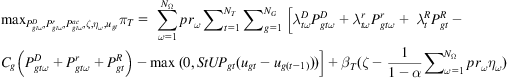
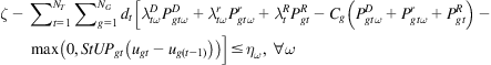
The objective function (4.10.1) comprises two terms: (1) The expected profit, which equals the revenues from the DA, RT, and bilateral reserve markets minus the production and start-up costs; and (2) the CVaR multiplied by a weighting factor βT, which allows the degree of risk aversion of the conventional power energy owner to be controlled.
In this model, the first-stage decision variable is the hourly bid of the energy volume ![]() of the thermal units while the second-stage decision variable is the RT output
of the thermal units while the second-stage decision variable is the RT output ![]() of the thermal units. Constraints (4.10.2)–(4.10.4) bind the maximum power capacity of each thermal unit. The actual total power generated by each thermal unit is expressed in constraint (4.10.5). Constraints (4.10.6) and (4.10.7) represent the ramp-up and ramp-down limits of each thermal unit, respectively. The production cost Cg of each thermal unit is expressed as a quadratic constraint (4.10.8). Constraint (4.10.9) enforces a nondecreasing offer curve. Constraint (4.10.10) constitutes the nonanticipativity conditions related to the decisions made in the first-stage. Constraints (4.10.11) and (4.10.12) are used to compute CVaR.
of the thermal units. Constraints (4.10.2)–(4.10.4) bind the maximum power capacity of each thermal unit. The actual total power generated by each thermal unit is expressed in constraint (4.10.5). Constraints (4.10.6) and (4.10.7) represent the ramp-up and ramp-down limits of each thermal unit, respectively. The production cost Cg of each thermal unit is expressed as a quadratic constraint (4.10.8). Constraint (4.10.9) enforces a nondecreasing offer curve. Constraint (4.10.10) constitutes the nonanticipativity conditions related to the decisions made in the first-stage. Constraints (4.10.11) and (4.10.12) are used to compute CVaR.
2. Renewable energy owner model
The model (4.11) to maximize the profit of a renewable energy owner is
(4.11.1)
(4.11.2)
(4.11.3)
(4.11.4)
(4.11.5)
(4.11.6)
(4.11.7)
(4.11.8)
(4.11.9)
(4.11.10)
where ![]() ,
, ![]() ,
, ![]() ,
,![]() ,
, ![]() , and
, and ![]() are the decision variables.
are the decision variables. ![]() represents the power offered by the renewable energy owner in the DA market at time period t.
represents the power offered by the renewable energy owner in the DA market at time period t. ![]() ,
, ![]() , and
, and![]() represent the positive deviation, negative deviation and total deviation of the renewable energy owner in the RT market at time period t.
represent the positive deviation, negative deviation and total deviation of the renewable energy owner in the RT market at time period t.
The random variables include ![]() ,
, ![]() , and
, and ![]() , where
, where ![]() is the actual renewable energy production at time period t. The variables, if augmented with a subscript
is the actual renewable energy production at time period t. The variables, if augmented with a subscript ![]() , represent their realization in a scenario
, represent their realization in a scenario ![]() .
.
The constants and parameters are ![]() ,
,![]() ,
, ![]() , and
, and ![]() , where
, where ![]() is the installed capacity of the wind power energy owner and
is the installed capacity of the wind power energy owner and ![]() is the risk aversion parameter of the conventional power energy owner.
is the risk aversion parameter of the conventional power energy owner.
The objective function (4.11.1) comprises two terms: (1) The expected profit, which equals the revenue from the DA market plus the revenue from positive energy deviations in the RT market minus the cost for negative energy deviations in the RT market and the cost in the bilateral reserve market; and (2) the CVaR multiplied by a weighting factor βW, which controls the degree of risk aversion of the wind energy owner.
Again in this model, the first-stage decision variable is the hourly bid of the energy volume ![]() of the renewable energy owner, whereas the second-stage variables are the RT energy deviations
of the renewable energy owner, whereas the second-stage variables are the RT energy deviations ![]() and
and ![]() of the owner. Constraint (4.11.2) limits the amount of renewable energy that can be traded in the DA market. Constraints (4.11.3)–(4.11.6) determine the total positive –and negative energy deviations incurred by the renewable energy owner per period and scenario. Constraint (4.11.7) constitutes the nonanticipativity conditions related to the decisions made in the first-stage. Constraint (4.11.8) enforces a nondecreasing offer curve. Constraints (4.11.9) and (4.11.10) are used to compute CVaR.
of the owner. Constraint (4.11.2) limits the amount of renewable energy that can be traded in the DA market. Constraints (4.11.3)–(4.11.6) determine the total positive –and negative energy deviations incurred by the renewable energy owner per period and scenario. Constraint (4.11.7) constitutes the nonanticipativity conditions related to the decisions made in the first-stage. Constraint (4.11.8) enforces a nondecreasing offer curve. Constraints (4.11.9) and (4.11.10) are used to compute CVaR.
The two models of conventional and renewable energy owners are connected through the reserve volumes ![]() and
and ![]() and the reserve clearing price
and the reserve clearing price ![]() in the bilateral reserve settlement. The total reserve volume, that is, the sum of reserve volumes
in the bilateral reserve settlement. The total reserve volume, that is, the sum of reserve volumes ![]() , of conventional energy owner should be equal to
, of conventional energy owner should be equal to ![]() .
.
3. Solving the matrix game
The discretization of the strategy variables ![]() s may cause loss or artificial creation of a Nash equilibrium [16]. To capture a possibly missing Nash solution, the standard discrete equilibrium condition (4.9) is loosened by
s may cause loss or artificial creation of a Nash equilibrium [16]. To capture a possibly missing Nash solution, the standard discrete equilibrium condition (4.9) is loosened by ![]() to yield an approximate Nash equilibrium.
to yield an approximate Nash equilibrium.
(4.12)
The matrix payoffs are suppliers’ profits from both the energy and bilateral reserve markets. These profits are obtained by solving the two-stage constrained stochastic programming problems described in model (4.10) and (4.11) for all strategy tuples in the increasing order of bidding price and energy. After the payoffs for each strategy tuple are obtained, the strategy tuples are examined for the Nash equilibrium condition (4.12). Ref. [16] presented a method to find an appropriate value of ε for determining an approximate Nash equilibrium.
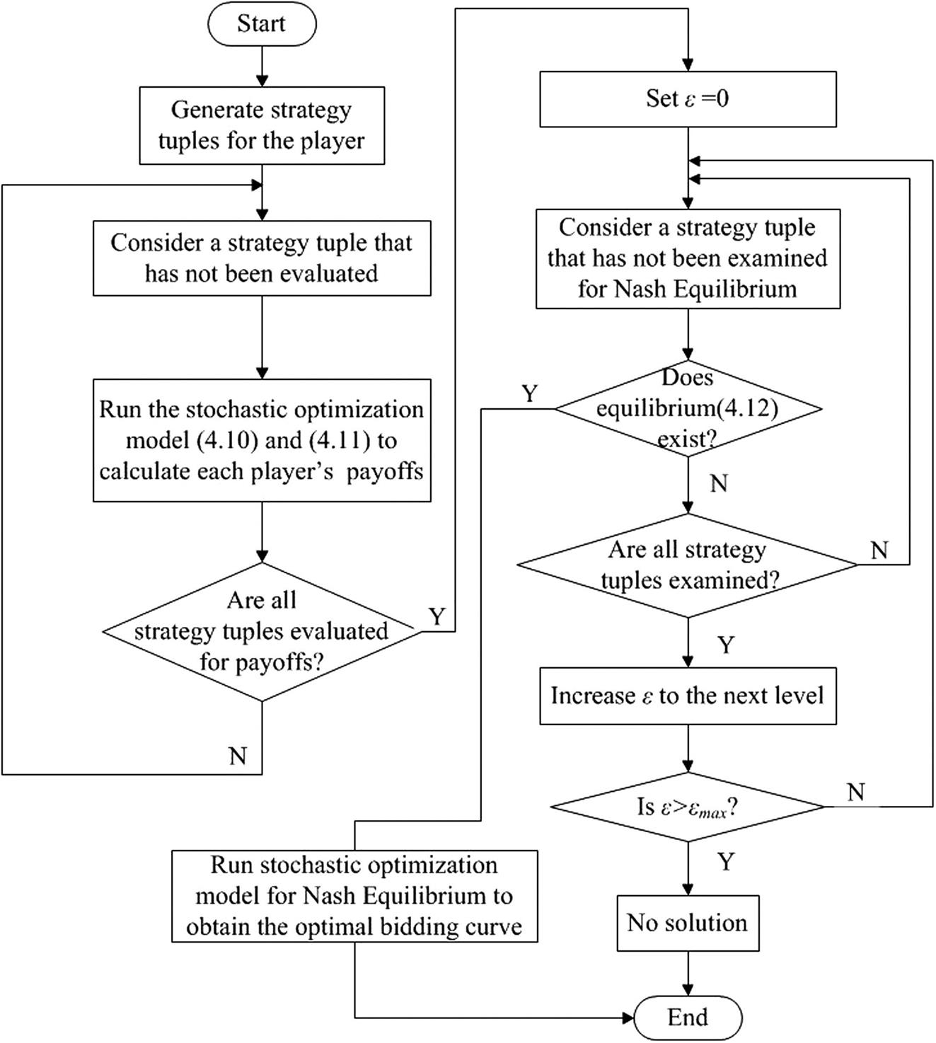
The complete solution process for trading renewable energy in both energy market and the bilateral reserve settlement is depicted in a flow chart in Fig. 4.8, which consists of two parts: obtaining the matrix payoffs by stochastic programming on the left-hand side and solving for the Nash equilibrium on the right-hand side. The strategies contain two variables: the reserve energy volume ![]() or
or ![]() that a conventional generating unit would like to offer or a renewable energy owner would like to buy, respectively, and the reserve clearing price
that a conventional generating unit would like to offer or a renewable energy owner would like to buy, respectively, and the reserve clearing price ![]() settled among conventional and renewable energy owners. These variables are discreated separately into a limited number of values within their limits defined by (4.5)–(4.7). A strategy tuple is then created by combining the values of these variables for all of the players in the game. For each strategy tuple, the stochastic optimization models (4.10) and (4.11) are executed for conventional and renewable energy owners, respectively, during which
settled among conventional and renewable energy owners. These variables are discreated separately into a limited number of values within their limits defined by (4.5)–(4.7). A strategy tuple is then created by combining the values of these variables for all of the players in the game. For each strategy tuple, the stochastic optimization models (4.10) and (4.11) are executed for conventional and renewable energy owners, respectively, during which ![]() (or
(or ![]() ) and
) and ![]() are constant values in this strategy tuple. Then, the Nash equilibrium condition is examined for each strategy tuple solved to determine which strategy tuple yields the maximum profits for both conventional and renewable energy owners. Finally, the stochastic programming is executed for the best strategy tuple, that is, the Nash equilibrium, to obtain the optimal bidding curve. The parameter εmax is relatively small compared with the expected profit obtained from the stochastic models, for example, 1% of the expected profit. If no solution is obtained from the search for the Nash equilibrium, wind energy owners will not bid reserve and conventional power energy owners will not offer reserve in the new bilateral reserve settlement.
are constant values in this strategy tuple. Then, the Nash equilibrium condition is examined for each strategy tuple solved to determine which strategy tuple yields the maximum profits for both conventional and renewable energy owners. Finally, the stochastic programming is executed for the best strategy tuple, that is, the Nash equilibrium, to obtain the optimal bidding curve. The parameter εmax is relatively small compared with the expected profit obtained from the stochastic models, for example, 1% of the expected profit. If no solution is obtained from the search for the Nash equilibrium, wind energy owners will not bid reserve and conventional power energy owners will not offer reserve in the new bilateral reserve settlement.
4.2.5.4 Case Study
Consider a game with two players: one thermal power plant with three units and one wind power plant. The installed capacities of the wind and thermal power plants are 100 and 140 MW, respectively. As there is only one thermal power energy owner in the market of providing the new type of bilateral reserve, the wind energy owner decides how much reserve it would like to buy from the thermal power energy owner and at what price. The thermal power energy owner decides the price of the reserved power and how much reserve it would like to sell. The thermal units’ operating characteristics are given in Table 4.3. The reserve price bid cap ccap is $1000/MW h in the reserve market. The ARIMA model is used to generate 5000 scenarios for wind power, DA price, and RT price predictions, respectively. Scenario reduction is then performed to reduce the scenarios of wind power, DA price, and RT price predictions to five each. Therefore, the final reduced scenario tree has 125 scenarios. The wind plant data is obtained from the National Renewable Energy Laboratory website [17]. The energy prices, including both the DA price and RT price, are obtained from the PJM website [11]. The risk aversion parameter is βT=βW=0.5. The confidence level is α=0.95. The maximum approximation parameter εmax (see Figure 4.8) is $10. For each thermal unit, three discrete reserve power volumes and three reserve clearing prices are generated. Assume that the reserve clearing price strategies are identical for the three units. A total of 81 strategy tuples are generated in this case study. The bidding curve for the wind energy owner is generated by solving the two-stage stochastic optimization problem (4.12) where the wind generation, RT price, and DA price are obtained through forecasting and scenario generation and reduction. The reserve price settled between wind and conventional power energy owners is obtained by using game theory. The expected profit is then calculated by applying the bidding curve obtained to the electricity market using real data obtained from the PJM market.
1. Case 1: RT price is lower than DA price
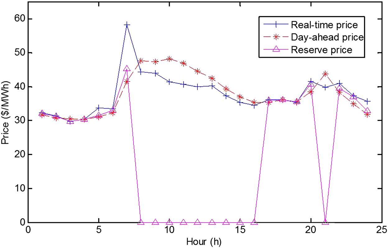
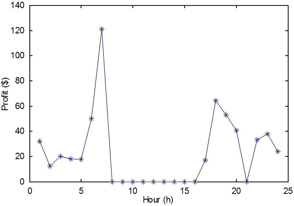
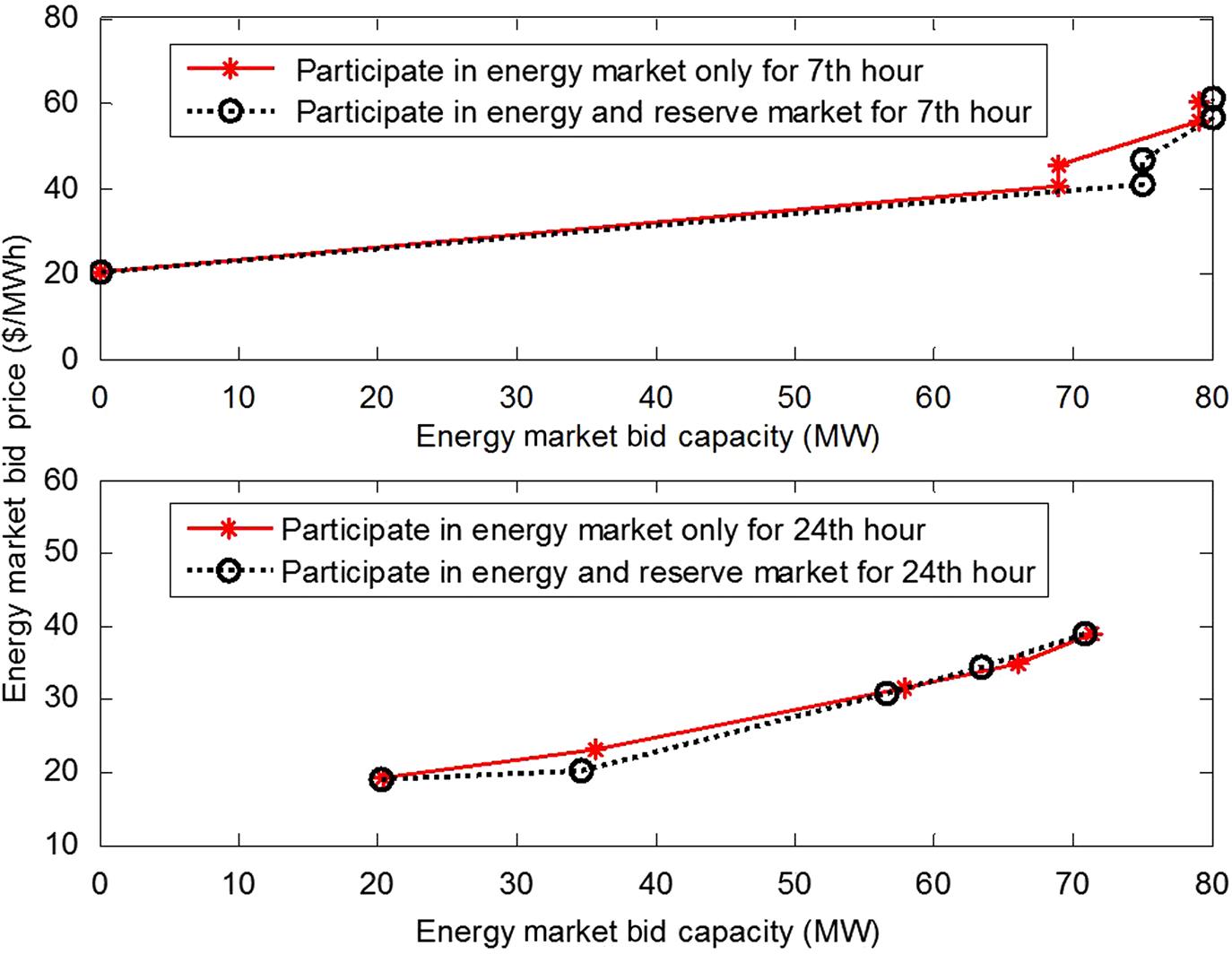
A day is selected in which the RT price has a low standard deviation; and during some hours, the RT price is lower than the DA price. The RT and DA prices obtained from the PJM market and the reserve price settled between wind and conventional power energy owners obtained from the proposed model are shown in Fig. 4.9. The total expected profits to be gained by the wind energy owner from participating in the energy market only and from participating in both the energy and bilateral reserve markets are shown in Fig. 4.10. The increased profit for the wind energy owner from playing a game with the thermal power energy owner in the bilateral reserve market to buy reserve energy is shown in Fig. 4.11. The energy market bidding curves of the wind energy owner participating in the energy market only and in both the energy and bilateral reserve markets for the 7th and 24th hours are shown in Fig. 4.12.
In this case, when the RT price is lower than the DA price, the thermal units would rather sell power in the DA market than the bilateral reserve market. The reserve price is then set to zero as there is no transaction of reserve in the bilateral reserve market. During hours when the RT price is higher than the DA price, the reserve price is settled between the RT and DA price. Thus, the wind energy owner could buy cheaper energy from the bilateral reserve market to gain a higher profit, as shown in Figs. 4.9 and 4.10. Buying energy from the bilateral reserve market has changed the wind bidding curve, as illustrated in Fig. 4.12. Compared with the case where the wind energy owner only participates in the energy market, if the wind energy owner participates in both the energy and bilateral reserve markets, it will bid at a higher price for low capacities and then decline its price to bid at a lower price for high capacities in the energy market. Moreover, the maximum capacity and price that the wind energy owner wishes to bid in the energy market are higher than if it only participated in the energy market. These observations are expected as the wind energy owner tends to first bid a higher price to cover the cost it will spend to buy reserve power and then to make more profit by selling more power.
2. Case 2: RT price has a high mean values and high standard deviations
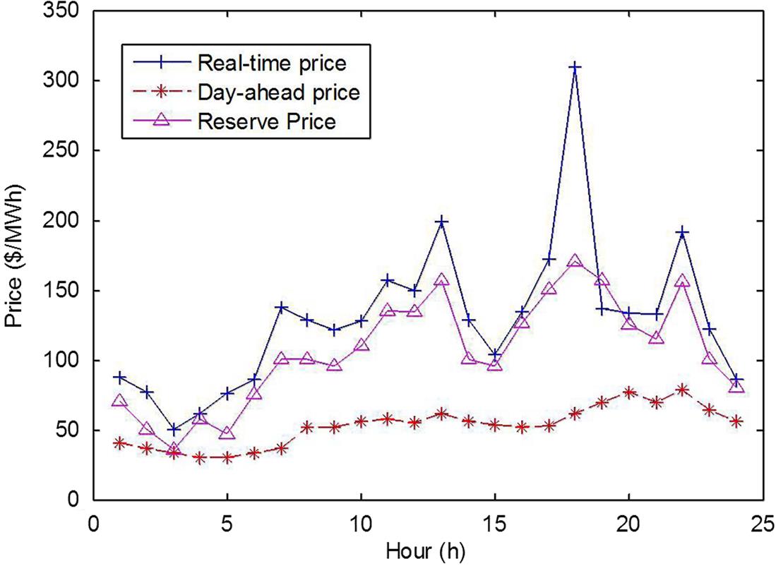
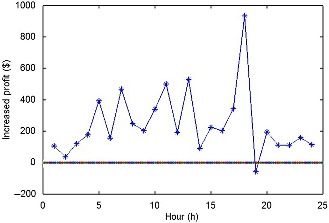
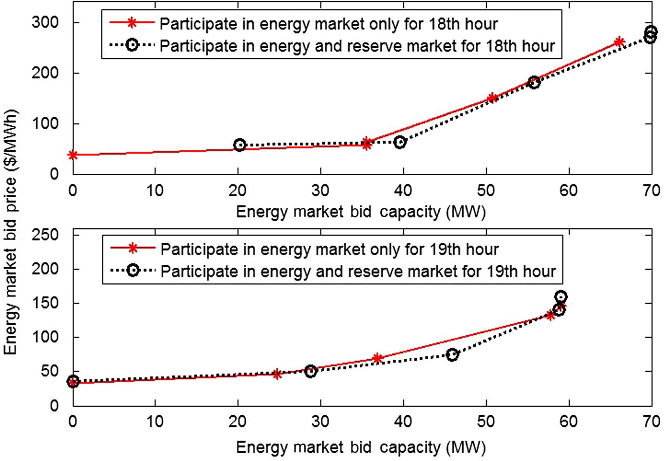
In this case, a day is chosen in which the mean value and standard deviation of the RT price is high. This means that the RT price is more difficult to predict for market participants. The RT, DA, and settled reserve prices are shown in Fig. 4.13. The total expected profits of the wind energy owner to gain from participating in the energy market and from participating in both the energy and bilateral reserve markets are shown in Fig. 4.14. The increased profit of the wind energy owner from buying reserve energy is shown in Fig. 4.15. The energy market bidding curves of the wind energy owner in participating in the energy market only and in both the energy and bilateral reserve markets for the 18th and 19th hours are shown in Fig. 4.16.
In this case, playing a game in the bilateral reserve market to buy reserve energy will not always benefit the wind power energy owner. In Fig. 4.13, the reserve price in the 19th hour is even higher than the RT price. Due to an inaccurate forecasting of the RT price, the wind energy owner buys expensive power from the bilateral reserve market, which results in a lower (negative) expected profit in that hour compared with the case where the wind energy owner does not participate in the bilateral reserve market, as shown in Fig. 4.15. However, most of the time, the wind energy owner gains more profits from playing the game in the bilateral reserve market. The bidding curves in the 18th and 19th hours in Fig. 4.16 show the same features as in Fig. 4.12.
The mean values of the increased profits of the wind power energy owner by playing the game in the bilateral reserve market are $22.5 in Case 1 and $244.8 in Case 2. A higher RT price results in more profit. The reserve price also has a tight correlation with the RT price and depends more on its fluctuations. A highly fluctuated RT price is more difficult to predict, which increases the risk of the wind energy owner losing money in the joint energy and bilateral reserve markets.
3. Impact of risk management
In the previous cases, both βW and βT were chosen to be 0.5. To study the impact of risk aversion, the expected profit of the wind energy owner and the CVaR for different βW are calculated for Case 2, where βW changes from 0 to 0.9 with an interval of 0.1. The influence of βT of the thermal units is also considered. Three curves are plotted in Fig. 4.17 for βT to be 0.1, 0.5, and 0.9, respectively, where each curve represents the relationship among the expected profit of the wind energy owner, CVaR, and βW.
As shown in Fig. 4.17, the three curves have the same trend. When βW increases, the value of CVaR increases, but the expected profit decreases. In the case of βT=0.5, the CVaR increases by approximately 43%, whereas the expected profit decreases by only 1.7% when βW increases from 0 to 0.9. When βT increases but βW remains constant, both the expected profit and CVaR increase. This is expected as when βT increases, the thermal units are willing to take less risk by selling more reserve to the wind energy owner, which increases the expected profit of the wind energy owner.
The impact of the risk aversion parameters for Cases 1 and 3 is similar to that of Case 2.


4.3 Price-Maker Models—MPEC Approach
4.3.1 Why Consider Wind Power Energy Owners as Price-Makers?
The previous section is based on the assumption that the renewable energy owner’s bidding strategies will not impact the market clearing prices. However, in real-world electricity market, this assumption is not always true.
As the Lerner index [18] has stated that the extent to which the bidding prices exceed the marginal cost is a measurement of market power
(4.13)
where L is the Lerner index, P is the market clearing price, and MC is the marginal cost of this power energy owner.
As we know, the renewable energy which has very low marginal costs and thus has nonnegligible market power and should be considered as price-makers.
4.3.2 Price-Maker Models—MPEC Approach
4.3.2.1 Introduction to MPEC
The strategic bidding model for a price-maker energy owner in the electricity market is different from that for a price-taker energy owner, as the price-maker energy owner has the market power to influence the market clearing prices; and the market clearing price, on the other hand, can influence the clearing power quantity of the price-maker energy owner [23]. To address this dependency, the problem can be formulated as a bilevel model. The upper-level model maximizes the profit of the price-maker energy owner from the electricity market. The lower level model represents the market clearing process.
The general formulation of a bilevel optimization problem (4.14) is the following:
(4.14.1)
Subject to:
(4.14.2)
(4.14.2)
(4.14.2)
Under the assumption that Karush–Kuhn–Tucker (KKT) conditions are necessary and sufficient for optimality in the lower level problem, we can employ them to replace condition (4.14.2) and transfer the bilevel problem into a singlelevel one (4.15) as follows:
(4.15.1)
Subject to
(4.15.2)
(4.15.3)
(4.15.4)
(4.15.5)
(4.15.6)
(4.15.7)
(4.15.8)
where λ and μ represent the dual variables associated to constraints ![]() and
and ![]() , respectively, in the lower level problem.
, respectively, in the lower level problem.
The lower level problem can be replaced by its first-order optimality condition, such as the widely used KKT condition. Thus, the original bilevel optimization problem can be transformed to a singlelevel problem, which is called a mathematical program with equilibrium constraints (MPEC). The MPEC approach has been widely used to obtain optimal bidding strategies for conventional energy owners. Readers who are interested in learning the MPEC approach application can find detailed information in Refs. [19–22].
4.3.2.2 Multistage Stochastic MPEC
The challenge to use the MPEC approach for modeling the bidding strategies of the price-maker renewable energy owners is the uncertainties involving in the modeling. Thus, the stochastic programming and MPEC approach will be combined together to model the bidding strategies of the price-maker renewable energy owner.
1. Uncertainties in the DA market
The main uncertainty in the DA market clearing process comes from the load and renewable energy forecast errors. The load and renewable energy forecast errors are unintentional and depend on the forecasting models. These forecast errors are handled by up and down reserves, which are scheduled as functions of the standard deviations of the forecasted renewable power and the total forecasted demand of the system are as follows:
(4.16)
where ![]() and
and ![]() are the total up and down reserve scheduled in a time period t, respectively.
are the total up and down reserve scheduled in a time period t, respectively. ![]() and
and ![]() are the standard deviation of the total forecasted demand and forecasted renewable power of the renewable generating unit j in a time period t, respectively.
are the standard deviation of the total forecasted demand and forecasted renewable power of the renewable generating unit j in a time period t, respectively. ![]() is a parameter decided by the system operator and is selected to be 3 in this chapter.
is a parameter decided by the system operator and is selected to be 3 in this chapter.
The reserve clearing process is assumed to be independent from the DA energy clearing and is modeled below:
(4.17.1)
(4.17.2)