Search in book...
Toggle Font Controls
Create new playlist

Name your new playlist

Playlist description (optional)
Sign In

Email address

Password

Forgot Password?

or

Continue with Facebook

Continue with Google
Sign Up

Full Name

Email address

Confirm Email Address

Password

or

Continue with Facebook

Continue with Google

Chapter 3

Optimal Procurement of Contingency and Load Following Reserves by Demand Side Resources Under Wind-Power Generation Uncertainty

Nikolaos G. Paterakis, Eindhoven University of Technology, Eindhoven, The Netherlands

Abstract

System operators must consider events that cause disturbances in the balance between the output of the generators and the load demand in their short-term operations. Transmission line failures, generating unit outages, and intrahour load deviations are such events. The means of confronting them is the scheduling and the deployment of reserves on a market basis. On top of these factors, the increasing penetration of renewables and especially wind-power generation has increased the frequency of deployment and the magnitude of required reserves. Traditionally, reserves have been procured by appropriately adjusting the output of the generating units; however, a broad range of demand-side resources are also qualified to provide ancillary services. The subject of this chapter is the development of a two-stage stochastic joint energy and reserve market structure that incorporates demand-side resources in order to procure the required reserve services in a reliable and economically optimal manner.

Keywords

Ancillary services; contingencies; demand response; reserves; two-stage stochastic programming; wind power; uncertainty

3.1 Introduction

The qualification and quantification of the appropriate ancillary services (ASs) in order to ensure the secure operation of the power system and the provision of uninterrupted and quality service to the consumers play a primordial role in the short-term operations of the System Operator (SO). More specifically, it should be guaranteed that sufficient capacity is kept in order to allow for corrective actions with the purpose of facing energy imbalances. Such imbalances may occur due to a generating unit outage or because of the failure of a transmission line. These events, which are commonly referred to as contingencies, constitute a severe jeopardy for the operation of the power system and should be tackled through the deployment of reserves to ensure the satisfaction of system constraints. Another source of imbalances is the deviation of the intrahour load demand from its forecasted value. In addition to that the large-scale penetration of renewable energy sources (RES), especially of wind-power generation, has resulted in an increased need for procuring reserves in order to accommodate the volatility in the power output of such resources.

Different SOs across the world utilize different definitions and procurement procedures as regards reserves [1,2]. Furthermore, apart from the more traditional reserve services, a new type of AS was recently introduced by Midcontinent Independent SO [3] and California Independent SO [4], namely the flexible ramping products. These services are designed to increase the robustness of the procurement of load-following reserves under uncertainty and are especially related to major ramping events caused by solar and wind-power resources.

It is nowadays a common ground that demand-side resources may be also deployed in order to provide system services, presenting significant potential technical and economic benefits, especially in the presence of high levels of RES penetration in the generation mix. The question this chapter deals with is whether demand response (DR) could facilitate the system operation when apart from system contingencies and intrahour load deviations, the SO must also confront the uncertainty in the production of wind farms.

Providing AS in a market framework primarily involves the solution of the unit commitment problem. Many different solution approaches have been proposed so far. A significant number of recent studies employ meta-heuristic techniques such as genetic and evolutionary algorithms [5–7], particle swarm optimization [8], tabu search and simulated annealing [9], as well as hybrid approaches [10]. Artificial intelligence methods such as fuzzy and expert systems [11], as well as neural networks [12] have been also used. Among the first methods applied to the solution of the unit commitment problem were the ones based on priority list [13] and mathematical programming. For instance, Lagrangian relaxation [14] is applied in Ref. [15] to a transient stability-constrained network structure. The Lagrangian relaxation method and its improved versions are also employed in Refs. [16,17]. The combination of Lagrangian relaxation with mixed-integer nonlinear programming is applied in Ref. [18]. Dynamic programming has been also extensively applied to the solution unit commitment problem in the past [19]. Mixed integer linear programming (MILP) approach may be currently considered as the state-of-the-art for the unit commitment problem solution, being almost exclusively employed in modern centralized market clearing engines and having been extensively studied in the literature [20–22]. A detailed discussion regarding the solution approaches of the unit commitment problem can be found in Ref. [23], while a recent review covering stochastic unit commitment is presented in Ref. [24].

Numerous technical studies that propose market designs in order to procure reserve services also exist. In Refs. [25,26], a stochastic security-constrained market-clearing procedure is developed, in which line and generator failures are taken into account through a set of preselected contingencies, while reserves are determined using the expected load not served as a penalty metric. A model to evaluate the economic impact of reserve provision under high wind-power generation penetration based on stochastic programming is provided in Ref. [27]. Moreover, the two-stage stochastic programming model presented in Ref. [28] considers the participation of DR providers in meeting the system constraints. A day-ahead market structure in which DR participation in contingency reserves is considered on the basis of bidding an offer curve representing the cost of rendering load curtailments available is also presented in Ref. [29].

A multi-agent based market model was proposed by Jafari et al. [30]. The day-ahead and several intraday markets, as well as a spot real-time market for energy and operating reserves are considered. However, in Ref. [30] involuntary load shedding is the only considered form of demand side participation. In Ref. [31], the operation of the power system in the presence of wind-power generation was analyzed on the basis of stochastic contingency analysis, neglecting the participation of DR resources. In Ref. [32], a switching operation between two separate energy markets named “conventional energy market” and “green energy market” was proposed, using a stochastic programming framework for profit maximization, without investigating the contribution of demand-side resources. Similar studies neglecting the contribution of DR to reserve procurement for managing uncertainties were conducted in Refs. [33–35]. It is worth mentioning though that the aforementioned studies made use of approaches to achieve computational efficiency. The computational efficiency of solving the problem of unit commitment under uncertainty was also the subject of Ref. [36].

Uncertainties stemming from wind-power generation and load demand were confronted by optimally scheduling hourly reserves using a security-constrained unit commitment in Ref. [37]. The dual decomposition algorithm was applied to solve the two-stage stochastic programming unit commitment problem in Ref. [38]. Jin et al. [39] modeled demand as a linear function of price in order to investigate the contribution of DR to reserves under significant wind-power generation penetration. Load uncertainty and generation unavailability were considered in Ref. [40] without accounting for RES uncertainty. Apart from the stochastic-programming-based literature referred above, there exist studies considering different uncertainty modeling frameworks such as probabilistic [41,42], rolling stochastic [43], and Monte Carlo criteria [44].

In this chapter a two-stage stochastic-programming-based joint energy and reserve market-clearing model within a MILP framework is developed. The uncertainty that is introduced by the penetration of wind-power generation, load deviations, and system contingencies is considered, so that economic optimality can be achieved. In order to guarantee the secure operation of the system, reserve services are procured from both generation and demand side resources which are represented by load serving entities (LSE). Two different time scales are introduced. The first stage of the model stands for the day-ahead market operation and is cleared on an hourly basis, while the second stage considers possible instances of uncertainty with a subhourly granularity.

3.2 Mathematical Model

3.2.1 Overview and Modeling Assumptions

The overview of the proposed model is portrayed in Fig. 3.1. The model is fed with a set of plausible wind-power generation scenarios and the technical and economic characteristics of the demand and generation side resources that might be employed in order to provide reserve services. The SO collects all the relevant information, as well as other system parameters (e.g., inelastic load forecast) and clears the market in a centralized fashion by solving the two-stage stochastic programming model. The model consists of two stages: The first stage represents the day-ahead market and involves variables and constraints that are not dependent on any specific scenario realization, while the second stage represents a possible instance of the day-ahead market in terms of uncertainty realization and comprises variables and constraints which are dependent on each individual scenario and its probability of occurrence. The first stage of the problem is cleared considering an hourly granularity, while the second stage is cleared using intrahour intervals. The time granularity of the second stage may be adjusted to the required time interval.

Figure 3.1 Overview of the market clearing model.

In this chapter, demand may belong to one of three categories. The first category of demand comprises the so-called inelastic loads. The consumption of the loads that fall in this category has to be fully satisfied under normal operating conditions and cannot be altered. Nonetheless, as a last resort and under a very high penalty, the SO may activate involuntary load shedding in order to satisfy the system constraints. Another type of loads is represented by LSE that contribute to load following reserves (LSE of type 1). Their consumption can be altered within prespecified limits in order to respond to wind-power generation fluctuations and intrahour load deviations. Finally, LSE, which are eligible for providing contingency reserves (LSE of type 2), stand for loads the consumption of which can be modified given that several constraints are satisfied. For example, it may be the case that there is a limited number of times that these resources may be called to respond and that every call has a specific maximum duration. More complex constraints (e.g., minimum time between two calls) and contract types can be easily integrated within the proposed methodology.

Two different types of reserve services are discerned. The first type is load following reserves that might be procured from both generating units and LSE that are committed to provide this service. More specifically, with the purpose of balancing intrahour and wind-power generation deviations, generating units provide synchronized up and down, as well as nonspinning reserves. The LSE of type 1 can provide this type of reserve by continuously adjusting their consumption upward or downward. The participation of the demand side in load following reserves is compensated at the utility value of the demand on the top of a cost paid for instructing them to be on stand-by.

In the case of a generating unit or a transmission line failure, a second type of reserves, namely contingency reserves, is activated. The energy deficit is counterbalanced by available synchronized and nonsynchronized units, or LSE that opt to provide this service. The LSE of type 2 that provide this service are compensated both at a value related to the period of the day they are called to provide this service, as well as for being on stand-by.

In order to facilitate the mathematical modeling of the problem, several assumptions are adopted. First of all, the only source of uncertainty taken into consideration is related to the wind production, since it is considered that the transmission line and unit contingencies on trial are perfectly known. The network constraints are considered in terms of a lossless linear representation, while active power losses may be included in the formulation as explained in Ref. [27]. Furthermore, the power output of units that become unavailable due to a contingency are instantly set to zero. Similarly, the active capacity of a transmission lines that trip is considered to be zero. Due to the short length of the horizon, it is assumed that units that fail are unavailable thereafter; though, it is possible that a line becomes available again within the examined horizon. Without loss of generality, the participation of wind-power producers is considered to be promoted by the SO. This means that as regards the market clearing procedure, wind energy is considered to be free of cost. In practice, it could be paid a regulated tariff out of the day-ahead market on the basis of the energy actually produced [27]. Regarding the modeling of the demand side resources, since in practice DR can respond in a few minutes [45], ramping constraints are not enforced for the LSE. Finally, only loads that are not subject to any resource offering scheme may incur involuntary load shedding.

3.2.2 Objective Function

$\begin{array}{l} EC & = \sum_{t_{1} \in T_{1}} {\sum_{i \in I} [\sum_{f \in F^{i}} (C_{i, f, t_{1}} \cdot b_{i, f, t_{1}}) + {SUC}_{i, t_{1}}^{1} + {SDC}_{i, t_{1}}^{1} + C_{i, t_{1}}^{R, DN} \cdot R_{i, t_{1}}^{R, DN} + C_{i, t_{1}}^{R, UP} \cdot R_{i, t_{1}}^{R, UP} + C_{i, t_{1}}^{R, NS} \cdot R_{i, t_{1}}^{R, NS}] \\ + \sum_{j_{1} \in J_{1}} (C_{j_{1}, t_{1}}^{DN, LSE 1} \cdot LSE 1_{j_{1}, t_{1}}^{DN} + C_{j_{1}, t_{1}}^{UP, LSE 1} \cdot LSE 1_{j_{1}, t_{1}}^{UP}) \\ + \sum_{j_{2} \in J_{2}} (C_{j_{2}, t_{1}}^{DN, LSE 2} \cdot LSE 2_{j_{2}, t_{1}}^{DN, con} + C_{j_{2}, t_{1}}^{UP, LSE 2} \cdot LSE 2_{j_{2}, t_{1}}^{UP, con})} \\ + \sum_{s \in S} π_{s} \sum_{t_{2} \in T_{2}} {\sum_{i \in I} [\sum_{f \in F^{i}} ({C'}_{i, f, t_{2}} \cdot r_{i, f, t_{2}, s}^{G}) + {CA}_{i, t_{2}, s}] \\ + \sum_{j_{1} \in J_{1}} λ_{j_{1}, t_{2}}^{LSE 1'} \cdot (LSE 1_{j_{1}, t_{2}, s}^{u} - LSE 1_{j_{1}, t_{2}, s}^{d}) \\ + \sum_{j_{2} \in J_{2}} λ_{j_{2}, t_{2}}^{LSE 2'} \cdot ψ_{j_{2}, t_{2}, s}^{LSE 2} + \sum_{w \in W} (\frac{V_{w, t_{2}}^{spill}}{Δ T_{1}} \cdot Δ T_{2} \cdot S_{w, t_{2}, s}) + \sum_{r \in R} (\frac{V_{r, t_{2}}^{LOL}}{Δ T_{1}} \cdot Δ T_{2} \cdot L_{r, t_{2}, s}^{shed})} \end{array}$ $\begin{array}{l} EC & = \sum_{t_{1} \in T_{1}} {\sum_{i \in I} [\sum_{f \in F^{i}} (C_{i, f, t_{1}} \cdot b_{i, f, t_{1}}) + {SUC}_{i, t_{1}}^{1} + {SDC}_{i, t_{1}}^{1} + C_{i, t_{1}}^{R, DN} \cdot R_{i, t_{1}}^{R, DN} + C_{i, t_{1}}^{R, UP} \cdot R_{i, t_{1}}^{R, UP} + C_{i, t_{1}}^{R, NS} \cdot R_{i, t_{1}}^{R, NS}] \\ + \sum_{j_{1} \in J_{1}} (C_{j_{1}, t_{1}}^{DN, LSE 1} \cdot LSE 1_{j_{1}, t_{1}}^{DN} + C_{j_{1}, t_{1}}^{UP, LSE 1} \cdot LSE 1_{j_{1}, t_{1}}^{UP}) \\ + \sum_{j_{2} \in J_{2}} (C_{j_{2}, t_{1}}^{DN, LSE 2} \cdot LSE 2_{j_{2}, t_{1}}^{DN, con} + C_{j_{2}, t_{1}}^{UP, LSE 2} \cdot LSE 2_{j_{2}, t_{1}}^{UP, con})} \\ + \sum_{s \in S} π_{s} \sum_{t_{2} \in T_{2}} {\sum_{i \in I} [\sum_{f \in F^{i}} ({C'}_{i, f, t_{2}} \cdot r_{i, f, t_{2}, s}^{G}) + {CA}_{i, t_{2}, s}] \\ + \sum_{j_{1} \in J_{1}} λ_{j_{1}, t_{2}}^{LSE 1'} \cdot (LSE 1_{j_{1}, t_{2}, s}^{u} - LSE 1_{j_{1}, t_{2}, s}^{d}) \\ + \sum_{j_{2} \in J_{2}} λ_{j_{2}, t_{2}}^{LSE 2'} \cdot ψ_{j_{2}, t_{2}, s}^{LSE 2} + \sum_{w \in W} (\frac{V_{w, t_{2}}^{spill}}{Δ T_{1}} \cdot Δ T_{2} \cdot S_{w, t_{2}, s}) + \sum_{r \in R} (\frac{V_{r, t_{2}}^{LOL}}{Δ T_{1}} \cdot Δ T_{2} \cdot L_{r, t_{2}, s}^{shed})} \end{array}$ (3.1)

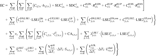
(3.1)

The objective function (3.1) stands for the minimization of the total expected cost (EC) of the system operation. The first line of (3.1) expresses the costs associated with energy provided from the generating units, the startup and shutdown costs, and the commitment of the units to provide reserves. The second and third lines represent the costs of scheduling reserves from the LSE of type 1 and type 2, respectively.

The rest of the objective function is scenario dependent, as indicated by the summation over the scenario index. Furthermore, in the second stage the intrahour intervals are taken into account, since a different set of time intervals is considered. The fourth line of the objective function takes into consideration the cost of changing the status of the generating units and the cost of actually deploying reserves from the generators. Similarly, the fifth line considers the cost of deploying reserves from the LSE of type 1. The sixth line stands for the cost of calling LSE of type 2 to provide contingency reserves. Finally, the last line takes into account the wind spillage cost and the EC of the energy not served to the inelastic loads.

$C_{i, f, t_{2}}^{'} = \frac{C_{i, f, t_{1}}}{Δ T_{1}} \cdot Δ T_{2} \forall i, f, t_{2} \in T_{2}^{in}, t_{1}$ $C_{i, f, t_{2}}^{'} = \frac{C_{i, f, t_{1}}}{Δ T_{1}} \cdot Δ T_{2} \forall i, f, t_{2} \in T_{2}^{in}, t_{1}$ (3.2)

(3.2)

$λ_{j_{1}, t_{2}}^{LSE 1^{'}} = \frac{λ_{j_{1}, t_{1}}^{LSE 1}}{Δ T_{1}} \cdot Δ T_{2} \forall i, f, t_{2} \in T_{2}^{in}, t_{1}$ $λ_{j_{1}, t_{2}}^{LSE 1^{'}} = \frac{λ_{j_{1}, t_{1}}^{LSE 1}}{Δ T_{1}} \cdot Δ T_{2} \forall i, f, t_{2} \in T_{2}^{in}, t_{1}$ (3.3)

(3.3)

$λ_{j_{2}, t_{2}}^{LSE 2^{'}} = \frac{λ_{j_{2}, t_{1}}^{LSE 2}}{Δ T_{1}} \cdot Δ T_{2} \forall i, f, t_{2} \in T_{2}^{in}, t_{1}$ $λ_{j_{2}, t_{2}}^{LSE 2^{'}} = \frac{λ_{j_{2}, t_{1}}^{LSE 2}}{Δ T_{1}} \cdot Δ T_{2} \forall i, f, t_{2} \in T_{2}^{in}, t_{1}$ (3.4)

(3.4)

Eqs. (3.2)–(3.4) are required in order to adjust the units of the marginal cost of the generating units and the utilities of the LSE. The cost unit is €/MW h which is suitable for the first stage of the problem in which the duration of the time interval is 1 h; however, in the second stage of the problem, intrahour intervals (min) are considered, and therefore, the cost units should be appropriately adjusted.

3.2.3 Constraints

3.2.3.1 First stage constraints

This section presents the first stage constraints of the optimization problem. These constraints involve only decision variables that do not depend on any specific scenario. Furthermore, the time dependence of variables refers to the time interval utilized in the first stage (i.e., hourly in this study) that is denoted by $t_{1} \in T_{1}$ $t_{1} \in T_{1}$ .

3.2.3.1.1 Generator output limits

$P_{i, t_{1}}^{sch} = \sum_{f \in F^{i}} b_{i, f, t_{1}} \forall i, t_{1}$ $P_{i, t_{1}}^{sch} = \sum_{f \in F^{i}} b_{i, f, t_{1}} \forall i, t_{1}$ (3.5)

(3.5)

$0 \leq b_{i, f, t_{1}} \leq B_{i, f, t_{1}} \forall i, f, t_{1}$ $0 \leq b_{i, f, t_{1}} \leq B_{i, f, t_{1}} \forall i, f, t_{1}$ (3.6)

(3.6)

$P_{i, t_{1}}^{sch} - R_{i, t_{1}}^{DN} \geq P_{i}^{\min} \cdot u_{i, t_{1}}^{1} \forall i, t_{1}$ $P_{i, t_{1}}^{sch} - R_{i, t_{1}}^{DN} \geq P_{i}^{\min} \cdot u_{i, t_{1}}^{1} \forall i, t_{1}$ (3.7)

(3.7)

$P_{i, t_{1}}^{sch} + R_{i, t_{1}}^{UP} \leq P_{i}^{\max} \cdot u_{i, t_{1}}^{1} \forall i, t_{1}$ $P_{i, t_{1}}^{sch} + R_{i, t_{1}}^{UP} \leq P_{i}^{\max} \cdot u_{i, t_{1}}^{1} \forall i, t_{1}$ (3.8)

(3.8)

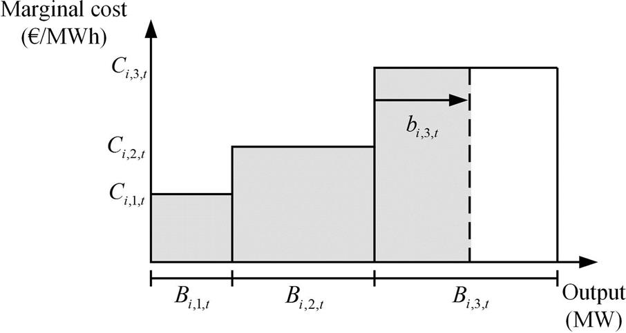
The generator bidding function is considered to be monotonically increasing and is approximated using a step-wise linear function as in Ref. [46]. This is enforced by (3.5) and (3.6). An example of a marginal cost function for a unit that offers its available energy in three blocks is illustrated in Fig. 3.2. Constraints (3.7) and (3.8) limit the output power of a generating unit, taking also into account the hourly scheduled up and down reserve margins.

Figure 3.2 Example of a step-wise linear bidding function.

3.2.3.1.2 Generator minimum up and down time constraints

$\sum_{τ = t_{1} - U T_{i}^{1} + 1}^{t_{1}} y_{i, τ}^{1} \leq u_{i, t_{1}}^{1} \forall i, t_{1}$ $\sum_{τ = t_{1} - U T_{i}^{1} + 1}^{t_{1}} y_{i, τ}^{1} \leq u_{i, t_{1}}^{1} \forall i, t_{1}$ (3.9)

(3.9)

$\sum_{τ = t_{1} - D T_{i}^{1} + 1}^{t_{1}} z_{i, τ}^{1} \leq 1 - u_{i, t_{1}}^{1} \forall i, t_{1}$ $\sum_{τ = t_{1} - D T_{i}^{1} + 1}^{t_{1}} z_{i, τ}^{1} \leq 1 - u_{i, t_{1}}^{1} \forall i, t_{1}$ (3.10)

(3.10)

Constraint (3.9) forces a unit to remain committed for at least ${UT}_{i}^{1}$ ${UT}_{i}^{1}$ hours once a startup decision is made ${(y}_{i, t_{1}}^{1} = 1)$ ${(y}_{i, t_{1}}^{1} = 1)$ , while (3.10) forces a unit to remain offline for at least ${DT}_{i}^{1}$ ${DT}_{i}^{1}$ hours once a shutdown decision is realized $(z_{i, t_{1}}^{1} = 1)$ $(z_{i, t_{1}}^{1} = 1)$ .

3.2.3.1.3 Unit commitment constraints

$y_{i, t_{1}}^{1} - z_{i, t_{1}}^{1} = u_{i, t_{1}}^{1} - u_{i, (t_{1} - 1)}^{1} \forall i, t_{1}$ $y_{i, t_{1}}^{1} - z_{i, t_{1}}^{1} = u_{i, t_{1}}^{1} - u_{i, (t_{1} - 1)}^{1} \forall i, t_{1}$ (3.11)

(3.11)

$y_{i, t_{1}}^{1} + z_{i, t_{1}}^{1} \leq 1 \forall i, t_{1}$ $y_{i, t_{1}}^{1} + z_{i, t_{1}}^{1} \leq 1 \forall i, t_{1}$ (3.12)

(3.12)

Eq. (3.11) enforces the startup and shutdown status change logic. The logical requirement that a unit cannot start up and shut down simultaneously during the same period is modeled using (3.12). Note that, these constraints indicate only the hour for which a startup or shutdown decision is taken but not the exact subhourly interval in which the startup or shutdown decision will actually occur.

3.2.3.1.4 Startup and shutdown costs

$SU C_{i, t_{1}}^{1} \geq SU C_{i} \cdot y_{i, t_{1}}^{1} \forall i, t_{1}$ $SU C_{i, t_{1}}^{1} \geq SU C_{i} \cdot y_{i, t_{1}}^{1} \forall i, t_{1}$ (3.13)

(3.13)

$SD C_{i, t_{1}}^{1} \geq SD C_{i} \cdot z_{i, t_{1}}^{1} \forall i, t_{1}$ $SD C_{i, t_{1}}^{1} \geq SD C_{i} \cdot z_{i, t_{1}}^{1} \forall i, t_{1}$ (3.14)

(3.14)

The cost that incurred when an off-line unit receives a command by the SO to start up or when an online unit is commanded to shut down is considered through constraints (3.13) and (3.14), respectively.

3.2.3.1.5 Ramp-up and ramp-down limits

$P_{i, t_{1}}^{sch} - P_{i, (t_{1} - 1)}^{sch} \leq Δ T_{1} \cdot R U_{i} \forall i, t_{1}$ $P_{i, t_{1}}^{sch} - P_{i, (t_{1} - 1)}^{sch} \leq Δ T_{1} \cdot R U_{i} \forall i, t_{1}$ (3.15)

(3.15)

$P_{i, (t_{1} - 1)}^{sch} - P_{i, t_{1}}^{sch} \leq Δ T_{1} \cdot R D_{i} \forall i, t_{1}$ $P_{i, (t_{1} - 1)}^{sch} - P_{i, t_{1}}^{sch} \leq Δ T_{1} \cdot R D_{i} \forall i, t_{1}$ (3.16)

(3.16)

In order to consider the effect of the ramp rates that limit the changes in the output of the generating units, constraints (3.15) and (3.16) are enforced. ${Δ T}_{1}$ ${Δ T}_{1}$ is the time length of the optimization interval of the first stage in minutes, for example, ${Δ T}_{1} = 60 \min$ ${Δ T}_{1} = 60 \min$ in the case of hourly granularity.

3.2.3.1.6 Generation side reserve scheduling

$0 \leq R_{i, t_{1}}^{UP} \leq T^{S} \cdot R U_{i} \cdot u_{i, t_{1}}^{1} \forall i, t_{1}$ $0 \leq R_{i, t_{1}}^{UP} \leq T^{S} \cdot R U_{i} \cdot u_{i, t_{1}}^{1} \forall i, t_{1}$ (3.17)

(3.17)

$0 \leq R_{i, t_{1}}^{DN} \leq T^{S} \cdot R D_{i} \cdot u_{i, t_{1}}^{1} \forall i, t_{1}$ $0 \leq R_{i, t_{1}}^{DN} \leq T^{S} \cdot R D_{i} \cdot u_{i, t_{1}}^{1} \forall i, t_{1}$ (3.18)

(3.18)

$0 \leq R_{i, t_{1}}^{NS} \leq T^{NS} \cdot R U_{i} \cdot (1 - u_{i, t_{1}}^{1}) \forall i, t_{1}$ $0 \leq R_{i, t_{1}}^{NS} \leq T^{NS} \cdot R U_{i} \cdot (1 - u_{i, t_{1}}^{1}) \forall i, t_{1}$ (3.19)

(3.19)

Constraints (3.17)–(3.19) impose limits on the procurement of reserves from the conventional generating units. Up and down spinning reserves and nonspinning reserves are defined by (3.17)–(3.19), respectively. Note that $T^{S}$ $T^{S}$ and $T^{NS}$ $T^{NS}$ denote the time in minutes during which the reserves should be fully deployed. The deployment time for each reserve type is defined by the rules that hold for each system. Note also that the aforementioned constraints are responsible for scheduling the total amount of reserve that is needed to cover all the imbalances considered in this study, that is, wind and load fluctuations, as well as contingencies.

$R_{i, t_{1}}^{UP} = R_{i, t_{1}}^{UP, load} + R_{i, t_{1}}^{UP, wind} + R_{i, t_{1}}^{UP, con} \forall i, t_{1}$ $R_{i, t_{1}}^{UP} = R_{i, t_{1}}^{UP, load} + R_{i, t_{1}}^{UP, wind} + R_{i, t_{1}}^{UP, con} \forall i, t_{1}$ (3.20)

(3.20)

$R_{i, t_{1}}^{DN} = R_{i, t_{1}}^{DN, load} + R_{i, t_{1}}^{DN, wind} + R_{i, t_{1}}^{DN, con} \forall i, t_{1}$ $R_{i, t_{1}}^{DN} = R_{i, t_{1}}^{DN, load} + R_{i, t_{1}}^{DN, wind} + R_{i, t_{1}}^{DN, con} \forall i, t_{1}$ (3.21)

(3.21)

$R_{i, t_{1}}^{NS} = R_{i, t_{1}}^{NS, load} + R_{i, t_{1}}^{NS, wind} + R_{i, t_{1}}^{NS, con} \forall i, t_{1}$ $R_{i, t_{1}}^{NS} = R_{i, t_{1}}^{NS, load} + R_{i, t_{1}}^{NS, wind} + R_{i, t_{1}}^{NS, con} \forall i, t_{1}$ (3.22)

(3.22)

Up spinning reserves, down spinning reserves and nonspinning reserves are scheduled in order to maintain the system balance during the actual operation of the power system that is disturbed due to positive or negative elastic or inelastic load deviations, wind ramp-ups and -downs, as well as contingency events. Up spinning reserves imply the increase in a synchronized unit’s power output, while down spinning reserves stand for the opposite. Nonspinning reserves are provided by nonsynchronized units as stated by (3.19). Eqs. (3.20)–(3.22) decompose the unit’s total scheduled up, down, or nonspinning reserves to different services that correspond to the different factors that can trigger the need of such reserves. The decomposition of reserves from the generation side is displayed in Fig. 3.3.

Figure 3.3 Reserve scheduling from generating units.

3.2.3.1.7 Wind-power scheduling

$0 \leq P_{w, t_{1}}^{WP, S} \leq P_{w}^{WP, \max} \forall w, t_{1}$ $0 \leq P_{w, t_{1}}^{WP, S} \leq P_{w}^{WP, \max} \forall w, t_{1}$ (3.23)

(3.23)

Typically, the wind-power generation scheduled in the day-ahead market is considered equal to its forecasted value. However, in this study, it is considered that the SO schedules the optimal amount of wind at each period $t_{1}$ $t_{1}$ according to the technoeconomic optimization within the limits imposed by (3.23). Several studies consider that the upper bound of wind-power scheduling in the day-ahead market is $\infty$ $\infty$ . However, in this study, the upper limit is considered equal to the installed capacity of each wind farm.

3.2.3.1.8 Load serving entities

It was stated before that the demand side can also contribute in reserves. In this study, two types of LSEs that are able to provide different reserve services are considered. First, the LSE of type 1 can provide up and down load following reserves in order to balance the wind fluctuations and the intrahour load deviations. Second, the LSE of type 2 may provide up and down reserve in order to confront contingencies. The two types of LSE are graphically illustrated in Figs. 3.4 and 3.5 in which the basic parameters of these loads are identified.

$LSE 1_{j_{1}, t_{1}}^{\min} \leq LSE 1_{j_{1}, t_{1}}^{sch} \leq LSE 1_{j_{1}, t_{1}}^{\max} \forall j_{1}, t_{1}$ $LSE 1_{j_{1}, t_{1}}^{\min} \leq LSE 1_{j_{1}, t_{1}}^{sch} \leq LSE 1_{j_{1}, t_{1}}^{\max} \forall j_{1}, t_{1}$ (3.24)

(3.24)

$0 \leq LSE 1_{j_{1}, t_{1}}^{UP} \leq LSE 1_{j_{1}, t_{1}}^{sch} - LSE 1_{j_{1}, t_{1}}^{\min} \forall j_{1}, t_{1}$ $0 \leq LSE 1_{j_{1}, t_{1}}^{UP} \leq LSE 1_{j_{1}, t_{1}}^{sch} - LSE 1_{j_{1}, t_{1}}^{\min} \forall j_{1}, t_{1}$ (3.25)

(3.25)

$LSE 1_{j_{1}, t_{1}}^{UP} = LSE 1_{j_{1}, t_{1}}^{UP, load} + LSE 1_{j_{1}, t_{1}}^{UP, wind} \forall j_{1}, t_{1}$ $LSE 1_{j_{1}, t_{1}}^{UP} = LSE 1_{j_{1}, t_{1}}^{UP, load} + LSE 1_{j_{1}, t_{1}}^{UP, wind} \forall j_{1}, t_{1}$ (3.26)

(3.26)

$0 \leq LSE 1_{j_{1}, t_{1}}^{DN} \leq LSE 1_{j_{1}, t_{1}}^{\max} - LSE 1_{j_{1}, t_{1}}^{sch} \forall j_{1}, t_{1}$ $0 \leq LSE 1_{j_{1}, t_{1}}^{DN} \leq LSE 1_{j_{1}, t_{1}}^{\max} - LSE 1_{j_{1}, t_{1}}^{sch} \forall j_{1}, t_{1}$ (3.27)

(3.27)

$LSE 1_{j_{1}, t_{1}}^{DN} = LSE 1_{j_{1}, t_{1}}^{DN, load} + LSE 1_{j_{1}, t_{1}}^{DN, wind} \forall j_{1}, t_{1}$ $LSE 1_{j_{1}, t_{1}}^{DN} = LSE 1_{j_{1}, t_{1}}^{DN, load} + LSE 1_{j_{1}, t_{1}}^{DN, wind} \forall j_{1}, t_{1}$ (3.28)

(3.28)

$\sum_{t_{1} \in T_{1}} LSE 1_{j_{1}, t_{1}}^{sch} \geq E_{j_{1}}^{req} \forall j_{1}$ $\sum_{t_{1} \in T_{1}} LSE 1_{j_{1}, t_{1}}^{sch} \geq E_{j_{1}}^{req} \forall j_{1}$ (3.29)

(3.29)

Figure 3.4 Load and reserve scheduling from LSE of type 1.

Figure 3.5 Load and reserve scheduling from LSE of type 2.

According to (3.24), the load may be scheduled within an upper and lower limit around its nominal value that defines its flexibility. The amount of up reserves that may be scheduled during a period t₁ are between zero and the margin that is defined by the difference between the scheduled and the minimum allowed load as stated in (3.25). These reserves are further decomposed into a component related to a reduction in order to balance wind fluctuations and a component that is related to balancing an intrahour deviation of the load as stated by (3.26). Similarly, the amount of down reserve that may be scheduled in each period is between zero and the capacity that is defined by the difference between the maximum allowed and the scheduled load, a fact that is stated by (3.27). The decomposition of down reserves in its components is realized by (3.28). Finally, in order to ensure that the LSE of type 1 energy needs are fulfilled during the horizon, despite the fact that it may be scheduled for partial curtailment in several periods, the energy requirement constraint (3.29) is enforced.

$LSE 2_{j_{2}, t_{1}}^{\min} \leq LSE 2_{j_{2}, t_{1}}^{sch} \leq LSE 2_{j_{2}, t_{1}}^{\max} \forall j_{2}, t_{1}$ $LSE 2_{j_{2}, t_{1}}^{\min} \leq LSE 2_{j_{2}, t_{1}}^{sch} \leq LSE 2_{j_{2}, t_{1}}^{\max} \forall j_{2}, t_{1}$ (3.30)

(3.30)

$0 \leq LSE 2_{j_{2}, t_{1}}^{UP, con} \leq LSE 2_{j_{2}, t_{1}}^{sch} - LSE 2_{j_{2}, t_{1}}^{\min} \forall j_{2}, t_{1}$ $0 \leq LSE 2_{j_{2}, t_{1}}^{UP, con} \leq LSE 2_{j_{2}, t_{1}}^{sch} - LSE 2_{j_{2}, t_{1}}^{\min} \forall j_{2}, t_{1}$ (3.31)

(3.31)

$0 \leq LSE 2_{j_{2}, t_{1}}^{DN, con} \leq LSE 2_{j_{2}, t_{1}}^{\max} - LSE 2_{j_{2}, t_{1}}^{sch} \forall j_{2}, t_{1}$ $0 \leq LSE 2_{j_{2}, t_{1}}^{DN, con} \leq LSE 2_{j_{2}, t_{1}}^{\max} - LSE 2_{j_{2}, t_{1}}^{sch} \forall j_{2}, t_{1}$ (3.32)

(3.32)

Similar to LSEs of type 1, the load of LSEs of type 2 may be scheduled within an upper and lower limit around its nominal value. This is enforced by (3.30). The up and down reserves that are scheduled by the LSEs of type 2 in order to confront system contingencies are defined by (3.31) and (3.32), respectively. This type of load is not subject to an energy requirement constraint due to the fact that it is paid to be curtailed for a prespecified number of periods.

3.2.3.1.9 Day-ahead market power balance

$\sum_{i \in I} P_{i, t_{1}}^{S} + \sum_{w \in W} P_{w, t_{1}}^{WP, S} = \sum_{r \in R} D_{r, t_{1}}^{1} + \sum_{j_{1} \in J_{1}} LSE 1_{j_{1}, t_{1}}^{sch} + \sum_{j_{2} \in J_{2}} LSE 2_{j_{2}, t_{1}}^{sch} \forall t_{1}$ $\sum_{i \in I} P_{i, t_{1}}^{S} + \sum_{w \in W} P_{w, t_{1}}^{WP, S} = \sum_{r \in R} D_{r, t_{1}}^{1} + \sum_{j_{1} \in J_{1}} LSE 1_{j_{1}, t_{1}}^{sch} + \sum_{j_{2} \in J_{2}} LSE 2_{j_{2}, t_{1}}^{sch} \forall t_{1}$ (3.33)

(3.33)

Eq. (3.33) enforces the market power balance. In other words, it states that the total generation of the conventional units and the total production of the wind farms must be equal to the demand of the inelastic load and the demand of the LSE of the two types at any given time interval $t_{1}$ $t_{1}$ . Although any scheme could be implemented within the proposed formulation, it is common not to enforce network constraints in the first stage of the problem [27].

3.2.3.2 Second-stage constraints

This section presents the second-stage constraints of the optimization problem. These constraints involve only decision variables that do depend on a specific scenario realization. Furthermore, the time dependence of variables refers to the time interval utilized in the second stage (i.e., subhourly intervals, e.g., 15 min) that is denoted by $t_{2} \in T_{2}$ $t_{2} \in T_{2}$ .

3.2.3.2.1 Generating units

Constraints (3.34)–(3.43) are related to the operation of the generation side in the light of each individual scenario outcome.

$P_{i, t_{2}, s}^{G} \geq P_{i}^{\min} \cdot u_{i, t_{2}, s}^{2} \forall i, t_{2}, s$ $P_{i, t_{2}, s}^{G} \geq P_{i}^{\min} \cdot u_{i, t_{2}, s}^{2} \forall i, t_{2}, s$ (3.34)

(3.34)

$P_{i, t_{2}, s}^{G} \leq P_{i}^{\max} \cdot u_{i, t_{2}, s}^{2} \forall i, t_{2}, s$ $P_{i, t_{2}, s}^{G} \leq P_{i}^{\max} \cdot u_{i, t_{2}, s}^{2} \forall i, t_{2}, s$ (3.35)

(3.35)

The minimum and maximum generation limits are also enforced in the second stage of the problem through (3.34) and (3.35).

$P_{i, t_{2}, s}^{G} - P_{i, (t_{2} - 1), s}^{G} \leq Δ T_{2} \cdot R U_{i} \forall i, t_{2}, s$ $P_{i, t_{2}, s}^{G} - P_{i, (t_{2} - 1), s}^{G} \leq Δ T_{2} \cdot R U_{i} \forall i, t_{2}, s$ (3.36)

(3.36)

$P_{i, (t_{2} - 1), s}^{G} - P_{i, t_{2}, s}^{G} \leq Δ T_{2} \cdot R D_{i} + N_{1} \cdot (1 - U C_{i, t_{2}}) \forall i, t_{2}, s$ $P_{i, (t_{2} - 1), s}^{G} - P_{i, t_{2}, s}^{G} \leq Δ T_{2} \cdot R D_{i} + N_{1} \cdot (1 - U C_{i, t_{2}}) \forall i, t_{2}, s$ (3.37)

(3.37)

As stated before, a ${Δ T}_{2}$ ${Δ T}_{2}$ -minute time interval is adopted in the second stage of the model constraints (3.36) and (3.37), which hold to limit the ramp-up and down of the units. As the ramp-up and -down rates of the generators are given in MW/min, the power output of a unit can change by its ramp-up or down rate multiplied by ${Δ T}_{2}$ ${Δ T}_{2}$ in each scenario. Note that constraint (3.37) is relaxed when the unit $i$ $i$ fails by using a sufficiently large value for the constant $N_{1}$ $N_{1}$ .

$\sum_{τ = t_{2} - \frac{U T_{i}^{2}}{Δ T_{2}} + 1}^{t_{2}} y_{i, τ, s}^{2} \leq u_{i, t_{2}, s}^{2} \forall i, t_{2}, s$ $\sum_{τ = t_{2} - \frac{U T_{i}^{2}}{Δ T_{2}} + 1}^{t_{2}} y_{i, τ, s}^{2} \leq u_{i, t_{2}, s}^{2} \forall i, t_{2}, s$ (3.38)

(3.38)

$\sum_{τ = t_{2} - \frac{D T_{i}^{2}}{Δ T_{2}} + 1}^{t_{2}} z_{i, τ, s}^{2} \leq 1 - u_{i, t_{2}, s}^{2} \forall i, t_{2}, s$ $\sum_{τ = t_{2} - \frac{D T_{i}^{2}}{Δ T_{2}} + 1}^{t_{2}} z_{i, τ, s}^{2} \leq 1 - u_{i, t_{2}, s}^{2} \forall i, t_{2}, s$ (3.39)

(3.39)

In the second stage of the problem, the minimum up and down times of the generating units are given in minutes. Thus, in (3.38) and (3.39) these times are divided by the duration of each interval ${Δ T}_{2}$ ${Δ T}_{2}$ in order to express the minimum up and down times in a number of intervals. Evidently, $U T_{i}^{2}$ $U T_{i}^{2}$ and $D T_{i}^{2}$ $D T_{i}^{2}$ must be integer multiples of ${Δ T}_{2}$ ${Δ T}_{2}$ .

$y_{i, t_{2}, s}^{2} + z_{i, t_{2}, s}^{2} \leq 1 \forall i, t_{2}, s$ $y_{i, t_{2}, s}^{2} + z_{i, t_{2}, s}^{2} \leq 1 \forall i, t_{2}, s$ (3.40)

(3.40)

$y_{i, t_{2}, s}^{2} - z_{i, t_{2}, s}^{2} = u_{i, t_{2}, s}^{2} - y_{i, (t_{2} - 1), s}^{2} \forall i, t_{2}, s$ $y_{i, t_{2}, s}^{2} - z_{i, t_{2}, s}^{2} = u_{i, t_{2}, s}^{2} - y_{i, (t_{2} - 1), s}^{2} \forall i, t_{2}, s$ (3.41)

(3.41)

Similarly to (3.11) and (3.12), constraints (3.40) and (3.41) ensure that the logic of unit commitment is preserved.

$SU C_{i, t_{2}, s}^{2} \geq SU C_{i} \cdot y_{i, t_{2}, s}^{2} \forall i, t_{2}, s$ $SU C_{i, t_{2}, s}^{2} \geq SU C_{i} \cdot y_{i, t_{2}, s}^{2} \forall i, t_{2}, s$ (3.42)

(3.42)

$SD C_{i, t_{2}, s}^{2} \geq SD C_{i} \cdot z_{i, t_{2}, s}^{2} \forall i, t_{2}, s$ $SD C_{i, t_{2}, s}^{2} \geq SD C_{i} \cdot z_{i, t_{2}, s}^{2} \forall i, t_{2}, s$ (3.43)

(3.43)

The startup and shutdown costs of the generators incurred in the second stage are considered using (3.42) and (3.43).

3.2.3.2.2 Wind spillage limits

$0 \leq S_{w, t_{2}, s} \leq P_{w, t_{2}, s}^{WP} \forall w, t_{2}, s$ $0 \leq S_{w, t_{2}, s} \leq P_{w, t_{2}, s}^{WP} \forall w, t_{2}, s$ (3.44)

(3.44)

For technical and economic reasons the SO may decide to spill a portion of available wind production to facilitate the operation of the power system. This is enforced by (3.44).

3.2.3.2.3 Involuntary-load shedding limits

$0 \leq L_{r, t_{2}, s}^{shed} \leq D_{r, t_{2}}^{2} \forall w, t_{2}, s$ $0 \leq L_{r, t_{2}, s}^{shed} \leq D_{r, t_{2}}^{2} \forall w, t_{2}, s$ (3.45)

(3.45)

As a last resort the SO may decide to shed a portion of the inelastic demand. This requirement is enforced by constraint (3.45).

3.2.3.2.4 Energy requirement constraint for LSE of type 1

$\sum_{t_{2} \in T_{2}} \frac{LSE 1_{j_{1}, t_{2}, s}^{ac}}{Δ T_{2}} \geq E_{j_{1}}^{req} \forall j_{1}, s$ $\sum_{t_{2} \in T_{2}} \frac{LSE 1_{j_{1}, t_{2}, s}^{ac}}{Δ T_{2}} \geq E_{j_{1}}^{req} \forall j_{1}, s$ (3.46)

(3.46)

Constraint (3.46) enforces the energy requirement constraint for the LSE of type 1 in each scenario. The division with the duration of the time interval $Δ T_{2}$ $Δ T_{2}$ is required in order to appropriately match the units of energy and power.

3.2.3.2.5 Reserve deployment from LSE of type 2

Eqs. (3.47)–(3.55) enforce several constraints related to the deployment of reserves from the LSE of type 2.

$LSE 2_{j_{2}, t_{2}, s}^{u, con} \leq N_{2} \cdot υ_{j_{2}, t_{2}, s}^{u} \forall j_{2}, t_{2}, s$ $LSE 2_{j_{2}, t_{2}, s}^{u, con} \leq N_{2} \cdot υ_{j_{2}, t_{2}, s}^{u} \forall j_{2}, t_{2}, s$ (3.47)

(3.47)

$LSE 2_{j_{2}, t_{2}, s}^{d, con} \leq N_{2} \cdot υ_{j_{2}, t_{2}, s}^{DN} \forall j_{2}, t_{2}, s$ $LSE 2_{j_{2}, t_{2}, s}^{d, con} \leq N_{2} \cdot υ_{j_{2}, t_{2}, s}^{DN} \forall j_{2}, t_{2}, s$ (3.48)

(3.48)

$υ_{j_{2}, t_{2}, s}^{LSE 2} = υ_{j_{2}, t_{2}, s}^{u} + υ_{j_{2}, t_{2}, s}^{DN} \forall j_{2}, t_{2}, s$ $υ_{j_{2}, t_{2}, s}^{LSE 2} = υ_{j_{2}, t_{2}, s}^{u} + υ_{j_{2}, t_{2}, s}^{DN} \forall j_{2}, t_{2}, s$ (3.49)

(3.49)

$υ_{j_{2}, t_{2}, s}^{u} + υ_{j_{2}, t_{2}, s}^{DN} \leq 1 \forall j_{2}, t_{2}, s$ $υ_{j_{2}, t_{2}, s}^{u} + υ_{j_{2}, t_{2}, s}^{DN} \leq 1 \forall j_{2}, t_{2}, s$ (3.50)

(3.50)

Constraints (3.47)–(3.50) are used in order force the LSE of type 2, once called, to provide only up or down contingency reserves. More specifically, (3.47) and (3.48) determine the amount of up and down reserve that may be deployed. The right hand side of these inequalities involves the multiplication of a sufficiently large constant $N_{2}$ $N_{2}$ with a binary variable that indicates whether an LSE of type 2 provides up or down reserve. If the LSE of type 2 is called in period $t_{2}$ $t_{2}$ then $υ_{j_{2}, t_{2}, s}^{LSE 2} = 1$ $υ_{j_{2}, t_{2}, s}^{LSE 2} = 1$ . The call implies that either up or down reserves are provided (either $υ_{j_{2}, t_{2}, s}^{u} = 1$ $υ_{j_{2}, t_{2}, s}^{u} = 1$ or $υ_{j_{2}, t_{2}, s}^{DN} = 1$ $υ_{j_{2}, t_{2}, s}^{DN} = 1$ ). These states are mutually exclusive, a fact that is expressed by (3.49) and (3.50).

$ψ_{j_{2}, t_{2}, s}^{LSE 2} - ζ_{j_{2}, t_{2}, s}^{LSE 2} = υ_{j_{2}, t_{2}, s}^{LSE 2} - υ_{j_{2}, (t_{2} - 1), s}^{LSE 2} \forall j_{2}, t_{2}, s$ $ψ_{j_{2}, t_{2}, s}^{LSE 2} - ζ_{j_{2}, t_{2}, s}^{LSE 2} = υ_{j_{2}, t_{2}, s}^{LSE 2} - υ_{j_{2}, (t_{2} - 1), s}^{LSE 2} \forall j_{2}, t_{2}, s$ (3.51)

(3.51)

$υ_{j_{2}, t_{2}, s}^{LSE 2} \geq ψ_{j_{2}, t_{2}, s}^{LSE 2} \forall j_{2}, t_{2}, s$ $υ_{j_{2}, t_{2}, s}^{LSE 2} \geq ψ_{j_{2}, t_{2}, s}^{LSE 2} \forall j_{2}, t_{2}, s$ (3.52)

(3.52)

$υ_{j_{2}, t_{2}, s}^{LSE 2} \geq ζ_{j_{2}, (t_{2} + 1), s}^{LSE 2} \forall j_{2}, t_{2}, s$ $υ_{j_{2}, t_{2}, s}^{LSE 2} \geq ζ_{j_{2}, (t_{2} + 1), s}^{LSE 2} \forall j_{2}, t_{2}, s$ (3.53)

(3.53)

Constraints (3.51)–(3.53) enforce the deployment logic of this type of resource.

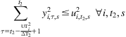
$\sum_{t_{2} \in T_{2}} ψ_{j_{2}, t_{2}, s}^{LSE 2} \leq N_{j_{2}}^{call} \forall j_{2}, t_{2}, s$ $\sum_{t_{2} \in T_{2}} ψ_{j_{2}, t_{2}, s}^{LSE 2} \leq N_{j_{2}}^{call} \forall j_{2}, t_{2}, s$ (3.54)

(3.54)

$\sum_{τ = t_{2} - \frac{T_{j_{2}}^{dur}}{Δ T_{2}} + 1}^{t_{2}} ψ_{j_{2}, τ, s}^{LSE 2} \geq υ_{j_{2}, t_{2}, s} \forall j_{2}, t_{2}, s$ $\sum_{τ = t_{2} - \frac{T_{j_{2}}^{dur}}{Δ T_{2}} + 1}^{t_{2}} ψ_{j_{2}, τ, s}^{LSE 2} \geq υ_{j_{2}, t_{2}, s} \forall j_{2}, t_{2}, s$ (3.55)

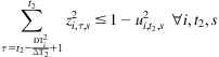
(3.55)

The deployment of demand side resources to provide reserve services may be subject to several rules, for example, maximum number of calls, duration of a call, and many more. Eq. (3.54) limits the maximum number of times each LSE of type 2 can be utilized to procure contingency reserves during the scheduling horizon. Finally, (3.55) constrains the maximum duration of each call to last at most $T_{j_{2}}^{dur}$ $T_{j_{2}}^{dur}$ periods.

3.2.3.2.6 Network constraints

$\begin{array}{l} \sum_{i \in N_{n}^{i}} P_{i, t_{2}, s}^{G} + \sum_{w \in N_{n}^{w}} (P_{i, t_{2}, s}^{WP} - S_{w, t_{2}, s}) + \sum_{n \in B_{b}^{nn}} f_{b, t_{2}, s} \\ = \sum_{n \in B_{b}^{n}} f_{b, t_{2}, s} + \sum_{r \in N_{n}^{r}} (D_{r, t_{2}}^{2} - L_{r, t_{2}, s}^{shed}) + \sum_{j_{1} \in N_{n}^{j_{1}}} SE 1_{j_{1}, t_{2}, s}^{ac} L + \sum_{j_{2} \in N_{n}^{j_{2}}} LSE 2_{j_{2}, t_{2}, s}^{a c} \forall b, (n, nn) \in B (n, nn), t_{2}, s \end{array}$ $\begin{array}{l} \sum_{i \in N_{n}^{i}} P_{i, t_{2}, s}^{G} + \sum_{w \in N_{n}^{w}} (P_{i, t_{2}, s}^{WP} - S_{w, t_{2}, s}) + \sum_{n \in B_{b}^{nn}} f_{b, t_{2}, s} \\ = \sum_{n \in B_{b}^{n}} f_{b, t_{2}, s} + \sum_{r \in N_{n}^{r}} (D_{r, t_{2}}^{2} - L_{r, t_{2}, s}^{shed}) + \sum_{j_{1} \in N_{n}^{j_{1}}} SE 1_{j_{1}, t_{2}, s}^{ac} L + \sum_{j_{2} \in N_{n}^{j_{2}}} LSE 2_{j_{2}, t_{2}, s}^{a c} \forall b, (n, nn) \in B (n, nn), t_{2}, s \end{array}$ (3.56)

(3.56)

$f_{b, t_{2}, s} = B_{b, n} \cdot (δ_{n, t_{2}, s} - δ_{nn, t_{2}, s}) \cdot L C_{b, t_{2}} \forall b, (n, nn) \in B (n, nn), t_{2}, s$ $f_{b, t_{2}, s} = B_{b, n} \cdot (δ_{n, t_{2}, s} - δ_{nn, t_{2}, s}) \cdot L C_{b, t_{2}} \forall b, (n, nn) \in B (n, nn), t_{2}, s$ (3.57)

(3.57)

$- f_{b}^{\max} \cdot L C_{b, t_{2}} \leq f_{b, t_{2}, s} \leq f_{b}^{\max} \cdot L C_{b, t_{2}} \forall b, t_{2}, s$ $- f_{b}^{\max} \cdot L C_{b, t_{2}} \leq f_{b, t_{2}, s} \leq f_{b}^{\max} \cdot L C_{b, t_{2}} \forall b, t_{2}, s$ (3.58)

(3.58)

$- π \leq δ_{n, t_{2}, s} \leq π \forall n, t_{2}, s$ $- π \leq δ_{n, t_{2}, s} \leq π \forall n, t_{2}, s$ (3.59)

(3.59)

$δ_{n, t_{2}, s} = 0 \forall t_{2}, s, if n \equiv ref$ $δ_{n, t_{2}, s} = 0 \forall t_{2}, s, if n \equiv ref$ (3.60)

(3.60)

In the second stage of the problem, the network constraints are taken into account using a lossless DC power flow formulation. More specifically, Eq. (3.56) stands for the power balance at each node of the system which states that the total power generated at each node by conventional units, the net production of wind farms plus the power injection from incoming transmission lines must equal the total net consumption of inelastic and elastic loads, as well as the power that is injected to outgoing transmission lines. The flow over a transmission line is defined by (3.57), while a power flow limit is set according to the maximum capacity of a transmission line by (3.58). In case of a transmission line failure, the active power flow through a transmission line is forced to zero. Finally, (3.59) and (3.60) state that the voltage angles must be bounded between $- π$ $- π$ and $π$ $π$ and that at the slack bus the voltage angle must be specified, respectively.

3.2.3.3 Linking constraints

The set of linking constraints bridges the day-ahead market decisions and the decisions made based on the outcome of each plausible scenario. As a result, the constraints pertaining this stage involve both scenario independent and scenario dependent decision variables. Linking constraints enforce the fact that reserves in the actual operation of the power system are no longer a stand-by capacity but are materialized as energy. To simplify the mathematical formulation presented below, the following should be noted: The equations that refer to reserve deployment by generating units hold only for units that are not under contingency. Furthermore, as long as there are no contingencies or wind/load deviations, the reserves provided by the demand side are also zero, and the relevant equations are not enforced. It should be also noted that the notation $t_{2} \in T_{2}^{in}$ $t_{2} \in T_{2}^{in}$ means that $t_{2}$ $t_{2}$ is a subhourly interval of the hour $t_{1}$ $t_{1}$ that appears in the same equation.

3.2.3.3.1 Additional cost due to change of commitment status of units

$C A_{i, t_{2}, s} = \sum_{t_{2} \in T_{2}} SU C_{i, t_{2}, s}^{2} - SU C_{i, t_{1}}^{1} + \sum_{t_{2} \in T_{2}} SD C_{i, t_{2}, s}^{2} - SD C_{i, t_{1}}^{1} \forall i, t_{2} \in T_{2}^{in}, t_{1}, s$ $C A_{i, t_{2}, s} = \sum_{t_{2} \in T_{2}} SU C_{i, t_{2}, s}^{2} - SU C_{i, t_{1}}^{1} + \sum_{t_{2} \in T_{2}} SD C_{i, t_{2}, s}^{2} - SD C_{i, t_{1}}^{1} \forall i, t_{2} \in T_{2}^{in}, t_{1}, s$ (3.61)

(3.61)

In the case of a difference occurring in the commitment status, a commitment scheduling change cost is charged through (3.61).

3.2.3.3.2 Generation side reserve deployment

$P_{i, t_{2}, s}^{G} = P_{i, t_{1}}^{sch} + r_{i, t_{2}, s}^{UP} + r_{i, t_{2}, s}^{NS} - r_{i, t_{2}, s}^{DN} \forall i, t_{2} \in T_{2}^{in}, t_{1}, s$ $P_{i, t_{2}, s}^{G} = P_{i, t_{1}}^{sch} + r_{i, t_{2}, s}^{UP} + r_{i, t_{2}, s}^{NS} - r_{i, t_{2}, s}^{DN} \forall i, t_{2} \in T_{2}^{in}, t_{1}, s$ (3.62)

(3.62)

$r_{i, t_{2}, s}^{UP} = r_{i, t_{2}, s}^{UP, load} + r_{i, t_{2}, s}^{UP, wind} + r_{i, t_{2}, s}^{UP, con} \forall i, t_{2}, s$ $r_{i, t_{2}, s}^{UP} = r_{i, t_{2}, s}^{UP, load} + r_{i, t_{2}, s}^{UP, wind} + r_{i, t_{2}, s}^{UP, con} \forall i, t_{2}, s$ (3.63)

(3.63)

$r_{i, t_{2}, s}^{DN} = r_{i, t_{2}, s}^{DN, load} + r_{i, t_{2}, s}^{DN, wind} + r_{i, t_{2}, s}^{DN, con} \forall i, t_{2}, s$ $r_{i, t_{2}, s}^{DN} = r_{i, t_{2}, s}^{DN, load} + r_{i, t_{2}, s}^{DN, wind} + r_{i, t_{2}, s}^{DN, con} \forall i, t_{2}, s$ (3.64)

..................Content has been hidden....................

You can't read the all page of ebook, please click here login for view all page.

Table of Contents for Chapter 3. Optimal Procurement of Contingency and Load Following Reserves by Demand Side Resources Under Wind-Power Generation Uncertainty

Create new playlist

Sign In

Sign Up