(4.17.3)
(4.17.4)
(4.17.5)
where ![]() and
and ![]() are the decision variables of the optimization problem (4.17).
are the decision variables of the optimization problem (4.17). ![]() and
and ![]() represent the up and down reserve scheduled for the conventional energy owner i in a time period t, respectively.
represent the up and down reserve scheduled for the conventional energy owner i in a time period t, respectively. ![]() and
and ![]() are the parameters which represent the maximum up and down reserve that can be provided by the conventional energy owner i, respectively.
are the parameters which represent the maximum up and down reserve that can be provided by the conventional energy owner i, respectively.
2. Uncertainties in the RT market
In the RT market clearing process, the main uncertainties come from the intentional misscheduling of load and wind power production deviation. If the power purchasers predict that the RT price will be lower than the DA price, they may intentionally underschedule load in the DA market and buy extra demand in the RT market at the RT price. Otherwise, if the power purchasers expect that the RT price will be higher than DA price, they may intentionally overschedule load and sell any extra energy procured in the DA market back to the system at the RT price. The behavior of these purchasers will increase the RT price volatility. For a wind power energy owner, the deviation of the actual production from that scheduled in the DA market will be balanced in the RT market. If the actual production is less than the DA scheduled, the wind energy owner will have to buy the deviated power at the RT price. Otherwise, the wind energy owner can bid the extra power into the RT market and get paid for the accepted power at the RT prices.
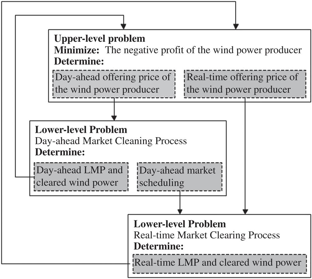
Overall, the problem to determine the optimal bidding strategy for a strategic wind power energy owner is formulated as a bilevel stochastic optimization model. Fig. 4.18 shows the structure of the stochastic bilevel model, which consists of an upper–lower problem and two lower level problems. The upper-level problem maximizes the total profit obtained by the wind power energy owner in both DA and RT markets to determine its optimal bidding curves in both markets. The maximal profit and the resulting bidding curves depend on the cleared information (LMPs and scheduled energy) in the DA and RT markets, which will be obtained in the lower level problems. One lower level problem collects the bidding information of each energy owner and runs the DA market clearing process to generate the DA LMPs and energy schedule for each energy owner. The other lower level problem is carried out after the DA clearing to deal with the RT energy deviation. This RT market clearing process depends not only on the RT offering curve of each energy owner but also on the DA energy schedule. Both the RT LMPs and RT energy schedule will be announced after the clearing.
4.3.3 Mathematical Formulation and Conversion
4.3.3.1 Bilevel Problem
1. Upper-level problem
The upper level problem (4.18) maximizing the total profit of the wind power energy owner in the DA and RT market is shown below:
(4.18.1)
(4.18.2)
(4.18.3)
(4.18.4)
(4.18.5)
where ![]() denotes the bus where the wind power generating unit w is located; and Ξ={
denotes the bus where the wind power generating unit w is located; and Ξ={![]() ,
,![]() ,
, ![]() ,
, ![]() , ΞD, ΞR } are the set of all decision variables of the problem (4.18), where ΞD and ΞR are the sets of all the decision variables in the lower level problems (4.19) and (4.20), respectively, and will be defined later. It should be noted that the total formulation for (4.18) consists of (4.18.1)–(4.18.5) and in addition the total formulations of (4.19) and (4.20).
, ΞD, ΞR } are the set of all decision variables of the problem (4.18), where ΞD and ΞR are the sets of all the decision variables in the lower level problems (4.19) and (4.20), respectively, and will be defined later. It should be noted that the total formulation for (4.18) consists of (4.18.1)–(4.18.5) and in addition the total formulations of (4.19) and (4.20). ![]() represents the offer price of block b of the wind generating unit j in a time period t in the DA market.
represents the offer price of block b of the wind generating unit j in a time period t in the DA market. ![]() represents the offer price of the wind generating unit j in a time period t in the RT market.
represents the offer price of the wind generating unit j in a time period t in the RT market.![]() and
and ![]() are auxiliary variables used to compute the CVaR. These variables, if augmented with a subscript
are auxiliary variables used to compute the CVaR. These variables, if augmented with a subscript ![]() , represent their realization in a scenario
, represent their realization in a scenario ![]() .
. ![]() and
and ![]() are constants which represent the cap bidding price in the DA and RT markets, respectively.
are constants which represent the cap bidding price in the DA and RT markets, respectively.
The objective function (4.18.1) minimizes the sum of two terms: (1) The negative expected profit of the wind power energy owner, which is the negative revenue obtained in the DA market plus the negative revenue from the RT market, and (2) the negative CVaRα multiplied by the weighting factor β. In (4.18.1), ![]() and
and ![]() are the variables determined in the lower level problem (4.19); while
are the variables determined in the lower level problem (4.19); while ![]() and
and ![]() are the variables determined in the lower level problem (4.20). The constraints (4.18.2) and (4.18.3) enforce the acceptable DA and RT bidding prices and nondecreasing DA bidding curves of the wind power energy owner. The constraints (4.18.4) and (4.18.5) are used to compute the CVaR, which is used in this paper as a measurement for risk. The CVaRα represents the expected profit associated with the (1−α)×100% worst scenarios. The weighting parameter β is set by the wind power energy owner to model the tradeoff between profit and risk. If the wind power energy owner is willing to gain less profit in order to bear less risk, it will select a higher value for β.
are the variables determined in the lower level problem (4.20). The constraints (4.18.2) and (4.18.3) enforce the acceptable DA and RT bidding prices and nondecreasing DA bidding curves of the wind power energy owner. The constraints (4.18.4) and (4.18.5) are used to compute the CVaR, which is used in this paper as a measurement for risk. The CVaRα represents the expected profit associated with the (1−α)×100% worst scenarios. The weighting parameter β is set by the wind power energy owner to model the tradeoff between profit and risk. If the wind power energy owner is willing to gain less profit in order to bear less risk, it will select a higher value for β.
2. Lower level problem—DA market clearing
The lower level problem (4.19) is formulated as follows to represent the DA market clearing process.
(4.19.1)
(4.19.2)
(4.19.3)
(4.19.4)
(4.19.5)
(4.19.6)
(4.19.7)
(4.19.8)
(4.19.9)
where ![]() is the bth element in the set WP(j,t); and ΞD={
is the bth element in the set WP(j,t); and ΞD={![]() ,
,![]() ,
,![]() ,
,![]() ,
, ![]() ,
,![]() ,
,![]() ,
,![]() ,
,![]() ,
,![]() ,
,![]() ,
,![]() ,
,![]() ,
,![]() ,
,![]() ,
,![]() } is the set of all decision variables of the problem (4.19). The decision variable set contains both primal and dual variables, where the dual variables are defined following the colon in each constraint.
} is the set of all decision variables of the problem (4.19). The decision variable set contains both primal and dual variables, where the dual variables are defined following the colon in each constraint. ![]() and
and ![]() represent the power produced in block b by the conventional power energy owner i and the wind power energy owner j in a time period t in the DA market, respectively.
represent the power produced in block b by the conventional power energy owner i and the wind power energy owner j in a time period t in the DA market, respectively. ![]() is the power bought by demand d in block l in a time period t in the DA market.
is the power bought by demand d in block l in a time period t in the DA market. ![]() is voltage angle of bus m in a time period t in the DA market.
is voltage angle of bus m in a time period t in the DA market. ![]() is the DA LMP at bus m in a time period t.
is the DA LMP at bus m in a time period t.![]() is the random variable which represents the offer price of block b of the conventional power energy owner i in a time period t in the DA market. Other variables include
is the random variable which represents the offer price of block b of the conventional power energy owner i in a time period t in the DA market. Other variables include ![]() and
and ![]() , where
, where ![]() is the capacity of block b of the conventional power energy owner i in a time period t in the DA market and
is the capacity of block b of the conventional power energy owner i in a time period t in the DA market and ![]() is the capacity of block l of the demand d in a time period t in the DA market. The constants are
is the capacity of block l of the demand d in a time period t in the DA market. The constants are ![]() ,
, ![]() ,
, ![]() , and
, and ![]() , where
, where ![]() is the imaginary part of the admittance of line m–n,
is the imaginary part of the admittance of line m–n, ![]() is the transmission capacity of lines m–n
is the transmission capacity of lines m–n ![]() and
and ![]() are the upper and lower limits of voltage magnitude of bus m, respectively.
are the upper and lower limits of voltage magnitude of bus m, respectively.
The objective function (4.19.1) minimizes the total cost of energy offered by both conventional and wind power energy owners minus the revenue from supplying demand in each period and each scenario. Eq. (4.19.2) enforces the DA power balance at each bus. The constraints (4.19.3)–(4.19.5) represent the limits of the power offered by the conventional and wind power units in each block. The constraint (4.19.6) represents the bounds of the demand in each block. The constraint (4.19.7) imposes the transmission capacity limits of each power line. The voltage angle limits of each bus are expressed in the constraint (4.19.8). The reference bus is selected in (4.19.9). Note that if the uncertainty of the bidding prices of the conventional power energy owner i is not considered, then ![]() ,
, ![]() .
.
3. Lower level problem—RT market clearing
The lower level problem (4.20) modeling the RT market clearing process is formulated below:
(4.20.1)
(4.20.2)
 (4.20.2)
(4.20.3)
(4.20.4)
(4.20.5)
(4.20.6)
(4.20.7)
(4.20.8)
(4.20.9)
(4.20.10)
(4.20.11)
(4.20.12)
(4.20.13)
where ΞR is the set of all primal and dual decision variables in the problem (4.20.1), where ΞR={![]() ,
, ![]() ,
, ![]() ,
, ![]() ,
, ![]() ,
, ![]() ,
, ![]() ,
,![]() ,
, ![]() ,
, ![]() ,
, ![]() ,
, ![]() ,
, ![]() ,
, ![]() ,
, ![]() ,
, ![]() ,
, ![]() ,
, ![]() ,
, ![]() ,
, ![]() ,
, ![]() ,
, ![]() ,
, ![]() ,
, ![]() ,
, ![]() ,
, ![]() ,
, ![]() }.
}. ![]() and
and ![]() represent the increased and decreased power of the conventional power energy owner i in a time period t in the RT market, respectively.
represent the increased and decreased power of the conventional power energy owner i in a time period t in the RT market, respectively. ![]() is the rescheduled power of the wind generating unit j in a time period t in the RT market.
is the rescheduled power of the wind generating unit j in a time period t in the RT market. ![]() is accepted deviation of the demand d in a time period t in the RT market.
is accepted deviation of the demand d in a time period t in the RT market. ![]() and
and ![]() represent up and down reserve deployed by the conventional power energy owner i in a time period t in the RT market, respectively.
represent up and down reserve deployed by the conventional power energy owner i in a time period t in the RT market, respectively. ![]() is voltage angle of bus m in a time period t in the RT market.
is voltage angle of bus m in a time period t in the RT market. ![]() is the RT LMP at bus m in a time period t.
is the RT LMP at bus m in a time period t.
The random variables include ![]() and
and ![]() , where
, where ![]() is the forecasted wind power production of the wind generating unit j in a time period t and
is the forecasted wind power production of the wind generating unit j in a time period t and ![]() is the forecasted deviation of demand d in a time period t.
is the forecasted deviation of demand d in a time period t.
The constants include ![]() ,
,![]() , and
, and ![]() , where
, where ![]() and
and ![]() represent the maximum increased and decreased power that can be provided by the conventional power energy owner i, respectively, and
represent the maximum increased and decreased power that can be provided by the conventional power energy owner i, respectively, and ![]() is the maximum power output of the conventional power energy owner i.
is the maximum power output of the conventional power energy owner i.
The objective function (4.20.1) minimizes the total cost of redispatching energy and deploying reserve minus the revenue from the deviation demand in each period and each scenario. Eq. (4.20.2) enforces the RT power balance at each bus. The constraints (4.20.3)–(4.20.6) limit the power of each conventional generator that can be sold into the RT market. The amount of wind power that can be sold in the RT market in each scenario is constrained by the forecasted wind power in the scenario, as described by (4.20.7). The bounds of the deviated demand in each scenario are represented by the constraint (4.20.8). The up and down reserves deployed are bounded by the scheduled up and down reserves in the DA market, respectively, as expressed in (4.20.9) and (4.20.10), respectively. The constraint (4.20.11) imposes the transmission capacity limits of each power line. The voltage angle limits of each bus are expressed in the constraint (4.20.12). The reference bus is selected in (4.20.13).
The wind power trading in the RT market is different from the conventional power energy owners due to the uncertainty in the wind power production. The wind power energy owner may fail to fulfill the productions settled in the DA market and is forced to correct its negative deviation in the RT market. Meanwhile, the wind power energy owner can bid the extra power into the RT market if the deviation is positive. The rescheduled wind power is constrained by (4.20.8) for both cases. As the DA market is cleared prior to the RT market, the decision variables ![]() and
and ![]() of the problem (4.18) and
of the problem (4.18) and ![]() ,
, ![]() , and
, and ![]() of the problem (4.19) are considered to be parameters in the problem (4.20).
of the problem (4.19) are considered to be parameters in the problem (4.20).
4.3.3.2 Model Conversion
The problem (4.19) is transferred by its KKT condition as follows where (4.21.5) is the same as (4.19.2):
(4.21.1)
(4.21.2)
(4.21.3)
(4.21.4)
(4.21.5)
(4.21.6)
(4.21.7)
(4.21.8)
(4.21.9)
(4.21.10)
(4.21.11)
(4.21.12)
(4.21.13)
(4.21.14)
(4.21.15)
(4.21.16)
where ⊥ denotes complementarity operation.
Similarly, the problem (4.20) is transferred by its KKT condition as follows where (4.22.8) is the same as (4.20.2):
(4.22.1)
(4.22.2)
(4.22.3)
(4.22.4)
(4.22.5)
(4.22.6)
(4.22.7)
(4.22.8)
 (4.22.8)
(4.22.9)
(4.22.10)
(4.22.11)
(4.22.12)
(4.22.13)
(4.22.14)
(4.22.15)
(4.22.16)
(4.22.17)
(4.22.18)
(4.22.19)
(4.22.20)
(4.22.21)
(4.22.22)
(4.22.23)
(4.22.24)
(4.22.25)
(4.22.26)
4.3.3.3 Reform MPEC as MILP
The MPEC problem having the objective function (4.19.1) and subject to the constraints (4.19.2)–(4.19.5), (4.21), and (4.22) is a nonlinear programming problem, where the nonlinearities come from the following three main sources. By linearizing the nonlinear terms, the MPEC problem is converted into a MILP problem, which can be solved effectively.
1. The ![]() term in (4.19.1).
term in (4.19.1).
According to (4.21.2), (4.21.3), (4.21.9), (4.21.10) and the strong duality theorem, this term can be linearized to (4.23).
(4.23)
 (4.23)
2. The ![]() term in (4.20.1).
term in (4.20.1).
Similar to (4.23), according to (4.22.3), (4.22.15), (4.22.16) and the strong duality theorem, this term can be linearized to (4.24).
(4.24)
 (4.24)
There is still a nonlinear term ![]() in (4.24). It can be linearized using the method in [24].
in (4.24). It can be linearized using the method in [24].
3. The MPEC model includes the nonlinear complementarity constraints (4.21.6)–(4.21.16) and (4.22.9)–(4.22.26). The complementarity constraint in the form of ![]() can be replaced by the following formulation.
can be replaced by the following formulation.
(4.25)
where M is a sufficiently large constant. Its value can be different for different complementarity constraints. Usually, M is set to be (dual variable + 1) × 100.
4.3.4 Case Study
The proposed model is tested using the IEEE Reliability Test System, which has 10 conventional power energy owners and one wind power energy owner. The detailed information for this test system can be found in Appendix. The total installed wind capacity is 1000 MW, which is approximately 23% of the total installed generation capacity in the system. In all case studies except for those explained specifically, all wind power generating units are located at bus 8 and the wind power energy owner is a strategic player in both the DA and the RT markets. The wind power data is obtained from the National Renewable Energy Laboratory website [17]. The historical data of the RT demand is obtained from the PJM market [11]. The parameters α and β in (4.18.1) are set to be 0.95 and 0, respectively. λCapD and λCapR are set to be $1000/MW h. In all of the case studies, the MILP problem is solved using Gurobi 5.5 in MATLAB [25].
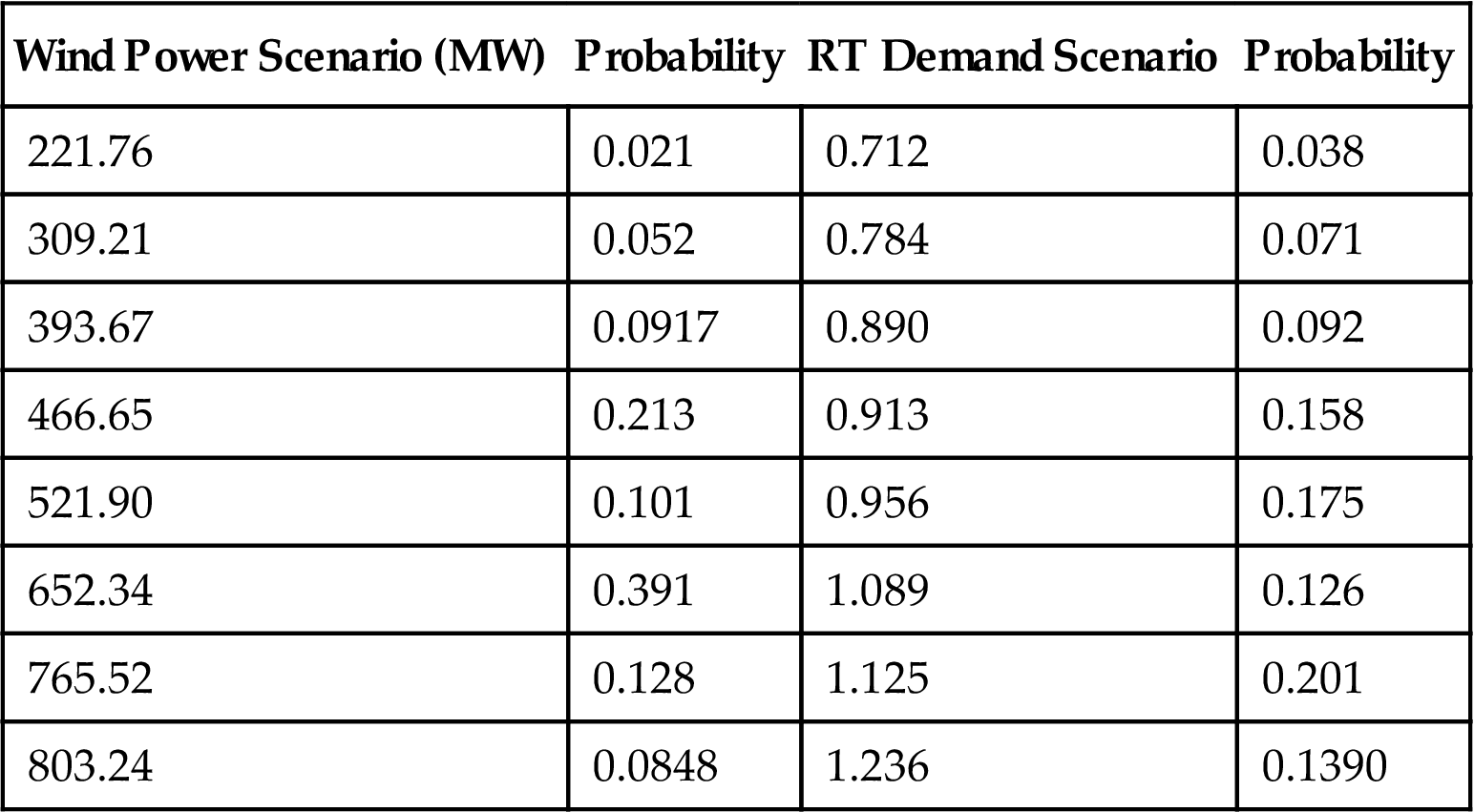
The ARIMA model is used to generate 5000 scenarios of wind power and RT demand respectively. Then the scenario reduction method is applied to reduce the number of scenarios for the wind power and RT demand. Table 4.4 lists the information (values and probabilities) of the resulting 8 wind power scenarios and 8 RT demand scenarios for a certain hour, where a RT demand scenario is described by the ratio of the forecasted RT demand to the DA demand.
1. The impact of wind power penetration level
In this study, the installed wind power capacity is changed from 200 MW (5% penetration) to 1600 MW (33% penetration) with an increment of 200 MW. No capacity limits are imposed on the transmission constraints. The DA and average RT LMPs of the 64 scenarios at bus 8 and the average selling price of the wind power energy owner are shown in Fig. 4.19 for different wind power penetration levels.
Due to the fact that wind power has no fuel cost, selling wind power into the market will lower the LMP. As shown in Fig. 4.19, both the DA LMP and the average RT LMP decrease as the penetration level of wind power increases. However, due to the effect of the uncertainties in the RT market, the RT LMP is more sensitive than the DA LMP to the changes of the demand and wind power supply. Therefore, the rate of decrease of the average RT LMP is much greater than that of the average DA LMP. When the penetration level is relatively low (5–15%), the average selling price of wind power increases with the increase of the wind power penetration level. At these penetration levels, as the RT LMP is much higher than the DA LMP, selling more wind power into the RT market will increase the average selling price. However, when the penetration level is relatively high (15–32%), the average selling price of wind power decreases with the increase of the wind penetration level. At these penetration levels, as the RT LMP decreases faster than the DA LMP and is even lower than the DA LMP when the penetration level becomes higher than 25%, selling the extra wind power into the RT market will decrease the average selling price. As can been seen more clearly from Fig. 4.20, the profit of the wind power energy owner in the DA market stays almost the same first, then increases dramatically, and finally stabilizes at a certain value when the penetration level increases. The cause of this result is explained below. When the penetration level of wind power is below 18%, the wind power energy owner does not have enough market power to influence the DA LMPs. Therefore, the DA LMP stays constant when the wind power penetration level changes within 18%. Moreover, when the wind power penetration level changes, the load demand in the DA market does not change. Therefore, the amounts of power bid into the DA market by the wind energy owner and the conventional generating units almost do not change. As a result, the profit of the wind energy owner in the DA market almost does not change. The results also show that the wind power energy owner intends to sell more power into the RT market to gain more profit because the RT LMP is higher than the DA LMP. This, however, results in a decline of the RT price. As the wind power penetration level goes higher, the DA LMP decreases dramatically; but the profit of the wind energy owner obtained from the DA market still increases because more power is sold into the DA market. However, the system’s ability to consume wind power in the DA market is limited. As the wind power penetration level reaches 25%, further increasing the penetration level only results in a slight change in the DA LMP and a slight increase in the wind power sold into the DA market. Therefore, the DA profit curve is almost constant as the wind power penetration level goes beyond 25%.
The profit in the RT market increases first until the penetration level reaches 18%. Beyond this penetration level, the RT profit decreases when the DA profit increases and then increases but is always below the DA profit when the penetration level exceeds 21%. As the RT price decreases to a certain level, the wind power energy owner will not sell all of its extra power into the RT market to prevent further decrease of the RT price and possible decrease of the total profit. As a result, some of the wind power generation capacity will be wasted as the wind power penetration level goes high. Therefore, it is important for the wind power energy owners to choose their installation capacities in a certain system. As Fig. 4.20 shows, the total profit of the wind energy owner increases with the wind penetration level.
2. The impact of transmission constraints
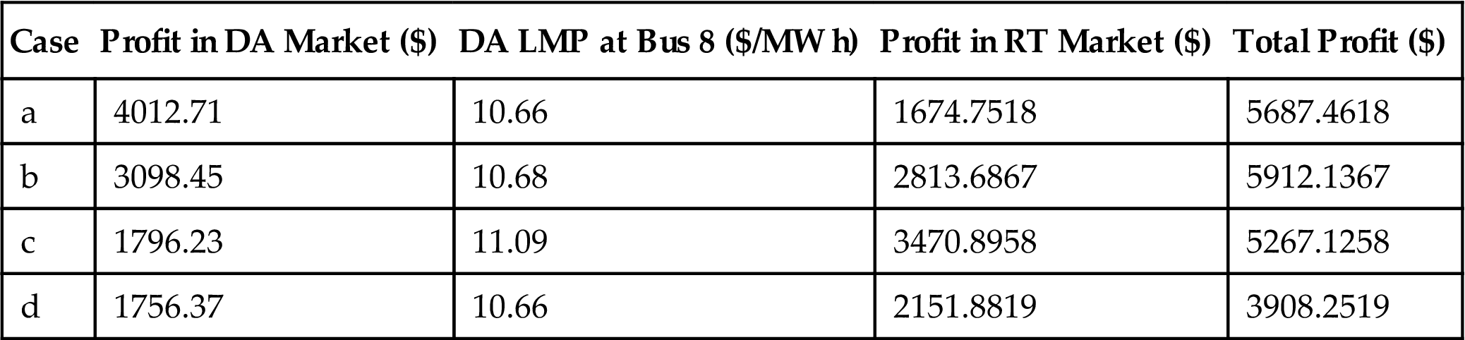
In this study, the wind power capacity is 1000 MW. The proposed model is solved to obtain the optimal bidding strategy for the wind energy owner for four cases: (a) no capacity limits are imposed on any transmission lines; and a capacity limit of (b) 190 MW, (c) 100 MW, and (d) 30 MW is imposed on the transmission line 8–9. Fig. 4.21 compares the RT LMPs at bus 8 in different scenarios for Cases (a), (b), and (c). Case (d) is not plotted because the RT LMPs of Cases (c) and (d) are the same. The profits of the wind power energy owner in the DA and RT markets, the total profit of the wind energy owner, and the DA LMP at bus 8 for different cases are given in Table 4.5.
When no capacity limits are imposed on the transmission lines, the power flow through line 8–9 is 75 MW in the DA market and maximally 292 MW in the RT market. As shown in Table 4.5, when the transmission capacity of line 8–9 is limited to 190 MW [Case (b)], the RT LMP in Scenario 64 is higher than that in Case (a). Although the amount of wind power sold into the DA market in Case (b) is lower than that in Case (a), the total profit in Case (b) is higher than that in Case (a) owing to the higher RT LMPs. Limiting the transmission capacity to 100 MW in Case (c) will further increase the RT LMP when compared to Case (b), as shown in Fig. 4.21. As a consequence, less amount of wind power will be sold in the DA market in Case (c) when compared with Cases (a) and (b). However, the increase of the RT LMP will not be able to compensate for the profit loss due to the decrease of the wind power sold in the DA market caused by the transmission congestion. In Case (d), the profit in the DA market increases slightly compared with Case (c) owing to the increase of the DA LMP. However, the total profit decreases dramatically compared with the previous three cases due to the small transmission capacity limit.
Based on the four case studies, it can conclude that transmission congestion sometimes can be beneficial to wind power energy owners and can be used as a strategic mechanism to increase their profits.
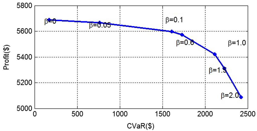
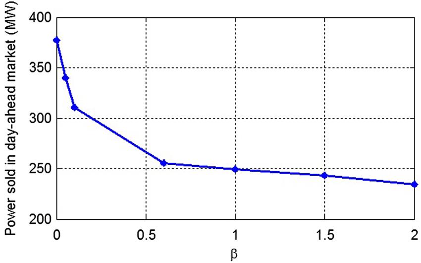
3. The impact of risk management
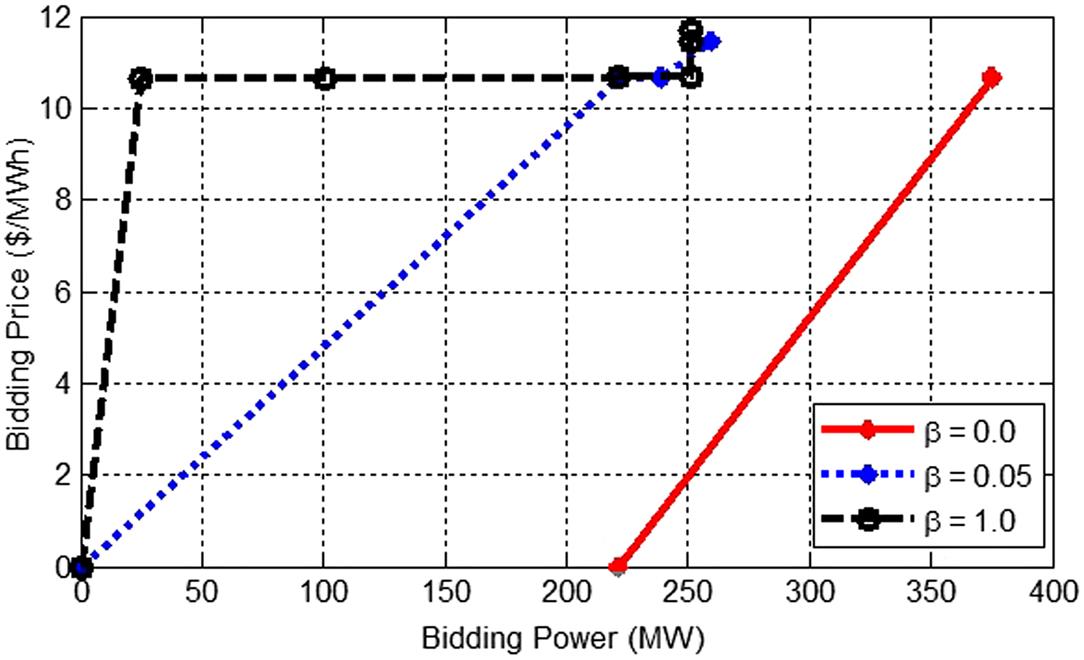
In this study, the installed wind power is 1000 MW. The proposed model is solved for different values of β in (3a). As shown in Fig. 4.22, the expected total profit of the wind power energy owner decreases and the CVaR increases with the increase of β. The wind bidding capacity in the DA market decreases when β increases, as plotted in Fig. 4.23. These results are expected. A higher β indicates that the wind power energy owner is willing to take less risk by selling less power into the DA market. As a consequence, the chance of the wind power energy owner to counter a negative deviation in the RT market decreases. The bidding curves of the wind power energy owner in the DA market for three selected values of β in Fig. 4.24 also show this trend: the bidding capacity decreases while the bidding price increases as β increases. Moreover, the expected total profit and bidding strategy are quite sensitive to the value of β when it is between 0 and 1.0, and its value should be selected carefully by the wind power energy owner. These results show the significance of risk management for the wind power energy owner to obtain the optimal bidding strategy.

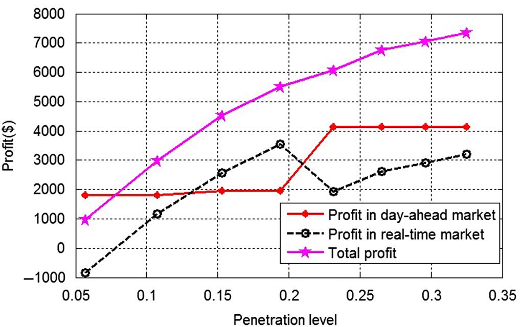

Table 4.5
Profits of the Wind Energy Owner and DA LMP at Bus 8 in Different Cases
| Case | Profit in DA Market ($) | DA LMP at Bus 8 ($/MW h) | Profit in RT Market ($) | Total Profit ($) |
| a | 4012.71 | 10.66 | 1674.7518 | 5687.4618 |
| b | 3098.45 | 10.68 | 2813.6867 | 5912.1367 |
| c | 1796.23 | 11.09 | 3470.8958 | 5267.1258 |
| d | 1756.37 | 10.66 | 2151.8819 | 3908.2519 |
4.4 Summary and Conclusion
This chapter starts with the introduction of the challenges and opportunities faced by the renewable energy owners participating in the electricity market. The main obstacle for renewable energy owners to compete with conventional power owners in the electricity market is the uncertainty in their production. However, as the PPA price goes down, the necessity for renewable energy owners to participate in the electricity market increases. Thus, appropriate models need to be built to help renewable energy owners benefit from electricity market.
In this chapter, the stochastic programming model is introduced to maximize the profit of the renewable energy owners and handle the uncertainties, for example, electricity market prices, renewable energy production, and others faced by renewable energy owners. The risk management CVaR is applied to managing the trade risk associated with uncertainties.
This chapter also considers two different types of renewable energy owners: Price-takers and price-makers. For the price-takers, their bidding strategies do not affect the market prices which can be considered as forecasted values in the stochastic model. Section 4.2.1 presented the basic stochastic programming model for this type of renewable energy owners and showed the readers how to build the bidding strategies. Section 4.2.2 introduced an approach to reduce the trading risks of the renewable energy owners by purchasing additional power from conventional energy owners. This approach has been analyzed using stochastic programming and game theory.
Section 4.3 proposed the model to solve the bidding strategies for the price-maker renewable energy owners whose bidding strategies have nonnegligible impact on the market clearing prices. The optimal bidding strategy of the renewable energy owner has been generated by a bilevel stochastic optimization model, which has been converted into a singlelevel MILP problem using the duality theory and KKT condition to facilitate solving the model.
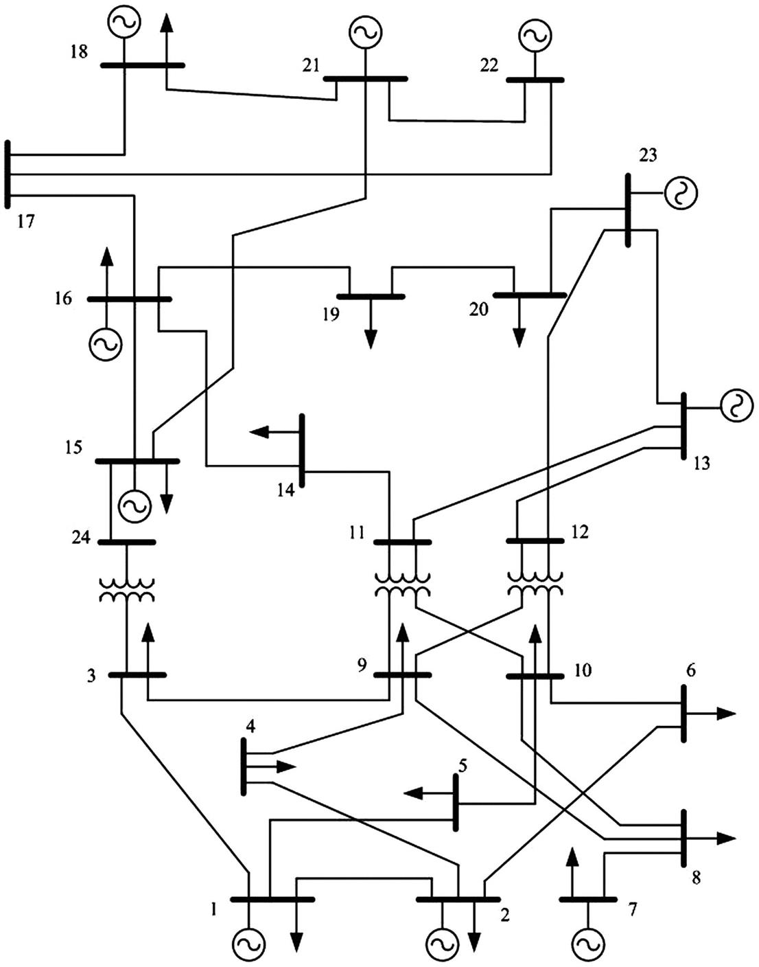
4.5 Appendix: IEEE Reliability Test System
This appendix illustrates the 24-bus system that used to exam the model in Section 4.3. This 24-bus system is based on the single-area version of the IEEE Reliability Test System [26]. See Figure 4.25.