
Optimum Sizing and Siting of Renewable-Energy-based DG Units in Distribution Systems
Amirsaman Arabali1, Mahmoud Ghofrani2, James B. Bassett2, My Pham2 and Moein Moeini-Aghtaei3, 1LCG Consulting, Los Altos, CA, United States, 2University of Washington, Bothell, WA, United States, 3Sharif University of Technology, Tehran, Iran
Abstract
The increasing demand for clean and nonfossil energy has escalated the integration of renewable power sources into the distribution system. Renewable distributed generators (DGs) have the potential to reduce the environmental impact when the integration into the distribution system is carefully optimized. However, serious technical issues will be raised when the integration is not properly implemented. This chapter presents optimal siting and sizing of renewable DG units within distribution systems. Both deterministic and probabilistic models of renewable-based DG units will be discussed in details along with characteristics of well-known renewable generators. The effects of DGs on distribution networks will be examined by defining several objective functions. The optimal DG siting and sizing problem will be introduced and formulated as an optimization problem and several solution methodologies will be discussed. Finally, a simple case study is provided that simulates the ideal placement of DG units within a distribution network.
Keywords
Renewable DG; DG placement; distribution losses; voltage stability; stochastic optimization
7.1 Introduction
The increasing demand for reliable power poses a challenge for traditional power generation models. As the demand increases, the consumption of finite resources and emission of climate altering CO2 escalate the urgency to integrate renewable power sources into the distribution system [1]. Distributed generators (DG) are relatively small power sources that can be powered by renewable and nonrenewable sources. Renewable-energy-based DGs have the potential to reduce the environmental impact of traditional power generation, but their integration into the distribution system must be carefully planned to optimize their benefit. The material in this chapter addresses the siting and sizing of DG units within distribution systems.
The power output of DG units ranges from a few kW to a few hundred kW and are classified in Table 7.1 by their output.
Table 7.1
Classification of DG Units by Power Output [2,3]
| Class | Size |
| Micro distributed generation | 1 W ≤ 5 kW |
| Small distributed generation | 5 kW ≤ 5 MW |
| Medium distributed generation | 5 MW ≤ 50 MW |
| Large distributed generation | 50 MW ≤ 500 MW |
The technologies associated with DG are broadly classified by their use of renewable or nonrenewable sources. Renewable sources include wind, solar photovoltaic (PV), solar thermal, hydro, biomass, geothermal, and tidal. Nonrenewable sources include reciprocating engines, gas turbines, combustion turbines, and fuel cells [3].
The economic impacts of using DG include the deferment of investment in building new power generation plants, and upgrading aging facilities. Certain DG technologies such as PV and wind have lower operation and maintenance (O&M) costs than traditional sources. In addition, reducing expenditures on fuel can provide enormous economic benefits to power providers. The diversification of the energy source profile may help insulate an economy to disruptions and fuel scarcity.
The environmental benefits of DG include reducing emissions of pollutants. This can have an indirect benefit in terms of reduced healthcare costs in high-pollution areas.
When implemented properly, there are technical benefits to the adoption of renewable DG within the power grid. These benefits include the minimization of system losses, improvement of the voltage profile, and enhanced system reliability, stability, and loadability. However, when not properly implemented, the technical benefits may become a liability. Stability issues, bidirectional power flow, harmonic instability, and islanding difficulties are challenges to overcome when integrating DG.
In the sections that follow, we will examine power generation models for renewable DG. We will examine the effects of DGs on the distribution network by considering the impact on voltage profile, power loss, reliability indices, economic cost and benefits, and voltage stability. Fault current, harmonic distortion, and reactive power supply will also be considered. We will then develop an objective function that can be used with a variety of solution techniques to model the siting and sizing of DG units within the distribution network. Finally, we will provide and discuss a case study that utilizes the theory to simulate the ideal placement of DG units.
7.2 Renewable-Energy-Based DG Models
For the purpose of predicting power output, power generation models of DG units can be categorized into deterministic and stochastic. Deterministic DG models are those in which the output can be highly controlled by increasing or decreasing the energy supply sources. Stochastic DG models have an inherent degree of variability due mostly to the unpredictability of regional weather conditions. For both types of DG models, it is desirable to model the net power output as a function of gross input. Gross input can be measured in terms of dollars per hour, cubic meters of gas per hour, incoming solar radiation per hour, or any other unit that accurately describes the operation of the facility. For stochastic models, gross input must include some form of probability distribution function (PDF) that models the unpredictable nature of the input. Net output is the electrical power that is available to the larger utility system.
7.2.1 Deterministic Models
Nonrenewable power generation technologies include reciprocating engines, gas turbines, combustion turbines, and others. For these technologies, the energy sources are not dependent upon fluctuations in the weather and therefore can be represented by deterministic models.
Renewable power generation technologies include geothermal and biomass. Because the energy supply in these technologies is stable and dispatchable to meet demand, they are considered to be deterministic, and their power models will not require PDFs. Geothermal and biomass power production will be analyzed in further detail.
7.2.1.1 Geothermal Models
The internal heat of the earth can be used to produce electricity through the use of steam turbines. The temperature ![]() at a depth
at a depth ![]() is given by
is given by ![]() , where
, where ![]() is the average temperature at the surface, and
is the average temperature at the surface, and ![]() is the temperature gradient. The temperature gradient is related to the heat flow Q and rock conductivity K by
is the temperature gradient. The temperature gradient is related to the heat flow Q and rock conductivity K by ![]() . The values for the temperature gradient and heat flow vary depending on the age of the geological formation, but are typically 20°C/km. Electricity production from geothermal sources are liquid based, where hot, compressed water fills the fractured and porous rocks of a reservoir. As the fluid moves upward toward the surface, the pressure decreases until the saturation pressure is reached corresponding to the geofluid temperature. The fluid begins to boil creating a two-phase liquid–vapor mixture that will flow through the upper section of the well. A separator will divert steam to turbine generators for electricity production and brine–water for either direct heating uses or will be returned to the reservoir through injection wells. After the steam has been used for electricity production, it passes through a condenser, is cooled, and is returned to the geothermal reservoir as shown in Fig. 7.1 [4].
. The values for the temperature gradient and heat flow vary depending on the age of the geological formation, but are typically 20°C/km. Electricity production from geothermal sources are liquid based, where hot, compressed water fills the fractured and porous rocks of a reservoir. As the fluid moves upward toward the surface, the pressure decreases until the saturation pressure is reached corresponding to the geofluid temperature. The fluid begins to boil creating a two-phase liquid–vapor mixture that will flow through the upper section of the well. A separator will divert steam to turbine generators for electricity production and brine–water for either direct heating uses or will be returned to the reservoir through injection wells. After the steam has been used for electricity production, it passes through a condenser, is cooled, and is returned to the geothermal reservoir as shown in Fig. 7.1 [4].
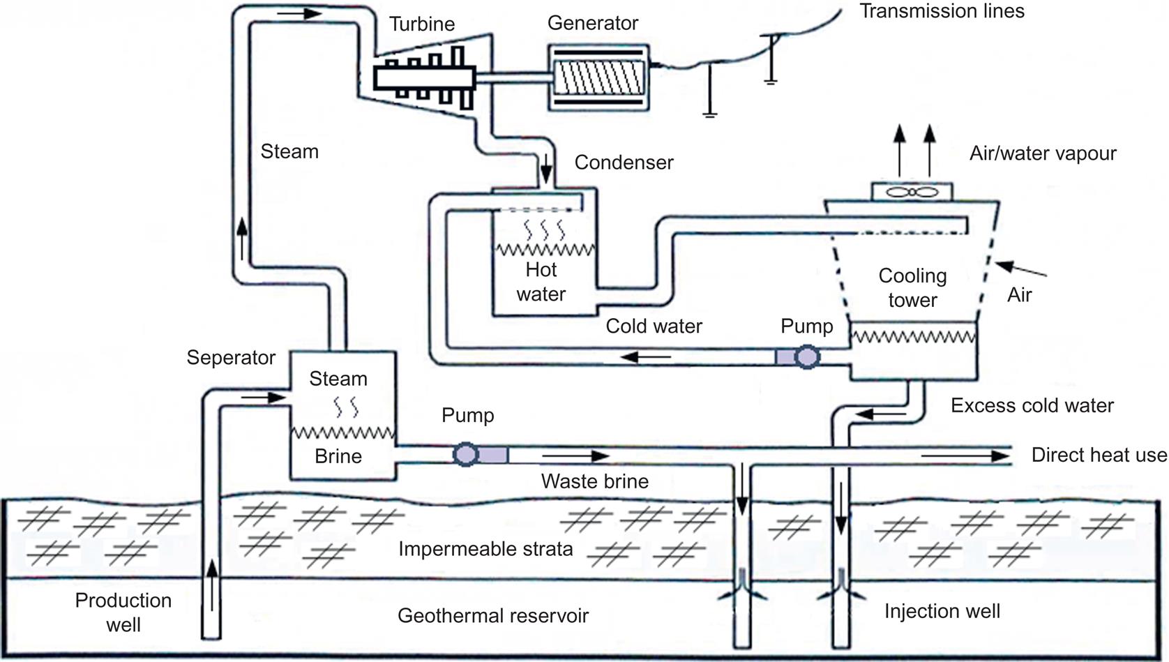
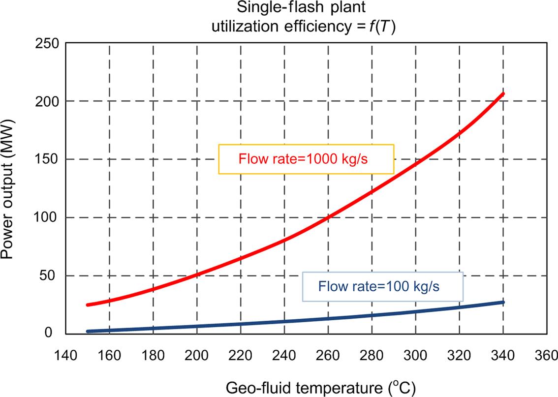
The potential power output of a geothermal plant depends primarily on two factors: The temperature of the geofluid and the fluid flow rate. Figs. 7.2 and 7.3 show these dependencies [5].

7.2.1.2 Biomass Models
Organic plant matter, known as biomass, can be converted to energy by burning, gasification, fermentation, or other processes. Wood products are the most common form of biomass power, but agricultural waste, yard-clippings, and municipal solid waste can also be used. To generate power, biomass is typically burned in a boiler, which produces high-pressure steam that is used to drive a turbine that generates electricity.
The power output potential for biomass depends on the heat content of the biomass fuels which is highly dependent on the plant species. Some combustion technologies can accept a wide range of biomass feedstock, while others require a much more homogenous feedstock. The heat content can also vary depending on the moisture content of the biomass fuel and the conversion technologies.
7.2.2 Stochastic Models
Two of the primary DG models that rely on variable input are wind energy and PV solar. Other renewable energy sources that have stochastic elements are solar thermal, microhydro, wave, and tidal. The wind energy and PV will be the focus of this chapter as they have seen a significant increase in deployment in recent years.
7.2.2.1 Wind Unit Models
The power generated by a wind turbine is calculated by a simple application of the kinetic energy equation ![]() through a cross sectional area A. The available power in Watts can be shown to be
through a cross sectional area A. The available power in Watts can be shown to be
(7.1)
where ![]() is the wind speed in meter per second (m/s),
is the wind speed in meter per second (m/s), ![]() is the density of air in kg/m3 (typically 1.225 kg/m3 at 15.55°C and 101,325 Pa),
is the density of air in kg/m3 (typically 1.225 kg/m3 at 15.55°C and 101,325 Pa), ![]() is the rotor diameter in m.
is the rotor diameter in m.
Clearly, as the wind speed increases, the power output will increase with the cube of the wind speed. This model must be adapted to account for cut-in speed, rated speed, and cut-out speed.
Low-wind speeds do not provide sufficient torque to the turbine blades to make them rotate. Power generation typically begins at wind speeds between 3 m/s and 4 m/s (6.71 and 8.95 mi/h). The wind speed at which power generation begins is called the cut-in speed.
As the wind speed exceeds the cut-in speed, power generation will rise steeply as a function of the cube of the wind speed. However, when the speed reaches a threshold, the wind turbine will reach its rated power output and will no longer increase its power as the velocity increases. This typically occurs between 12 m/s and 17 m/s (26.84 and 38.03 m/h). With large turbines, the wind power is usually maintained at a constant level by adjusting the angle of the blades.
As the speed increases above the rated speed, there is a danger that excessive forces will cause damage to the turbine. A braking system will engage and bring the rotor to a standstill. This occurs at the cut-out speed which is typically around 25 m/s (Fig. 7.4).

Energy production, measured in kW h, is ![]() . Since the power output of a wind turbine depends on the wind speed, predicting energy production requires the use of PDF to account for the variances in wind speed in time. There are two commonly used PDFs that are used to describe wind velocity variation: The normal (Gaussian) distribution and the Weibull distribution. The Weibull distribution is often a better fit for modeling wind speeds due to the asymmetry of measured distributions.
. Since the power output of a wind turbine depends on the wind speed, predicting energy production requires the use of PDF to account for the variances in wind speed in time. There are two commonly used PDFs that are used to describe wind velocity variation: The normal (Gaussian) distribution and the Weibull distribution. The Weibull distribution is often a better fit for modeling wind speeds due to the asymmetry of measured distributions.
The Weibull PDF applied to wind speeds is defined as
(7.2)
where ![]() is the shape factor,
is the shape factor, ![]() is the scale factor, and
is the scale factor, and ![]() is a vector of the measured wind speeds.
is a vector of the measured wind speeds.
The value of the shape factor ![]() determines the width of the wind speed distribution around the average. Smaller values indicate a relatively wider wind speed distribution, while a larger indicates the opposite. The scale factor
determines the width of the wind speed distribution around the average. Smaller values indicate a relatively wider wind speed distribution, while a larger indicates the opposite. The scale factor ![]() defines where the majority of the distribution lies and how stretched out the distribution is.
defines where the majority of the distribution lies and how stretched out the distribution is.
Fig. 7.5 shows a Weibull PDF for wind speed data collected during a 1-year period in Gilbert, IA and includes the shape and scale factors. MATLAB was used to analyze the data.
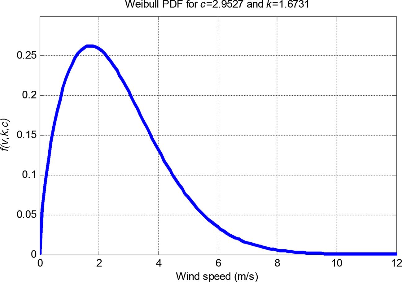
Fig. 7.6 shows the fitted Weibull PDF with c=5.0298, k=1.9579 compared to the empirical PDF plotted using historical hourly wind speed for the Ames site. The Weibull curve fitting is used to obtain the scale and shape factors using historical wind speed data. As shown, the fitted Weibull PDF is a suitable fit and an appropriate probabilistic model for the wind speed data.

7.2.2.2 PV Unit Models
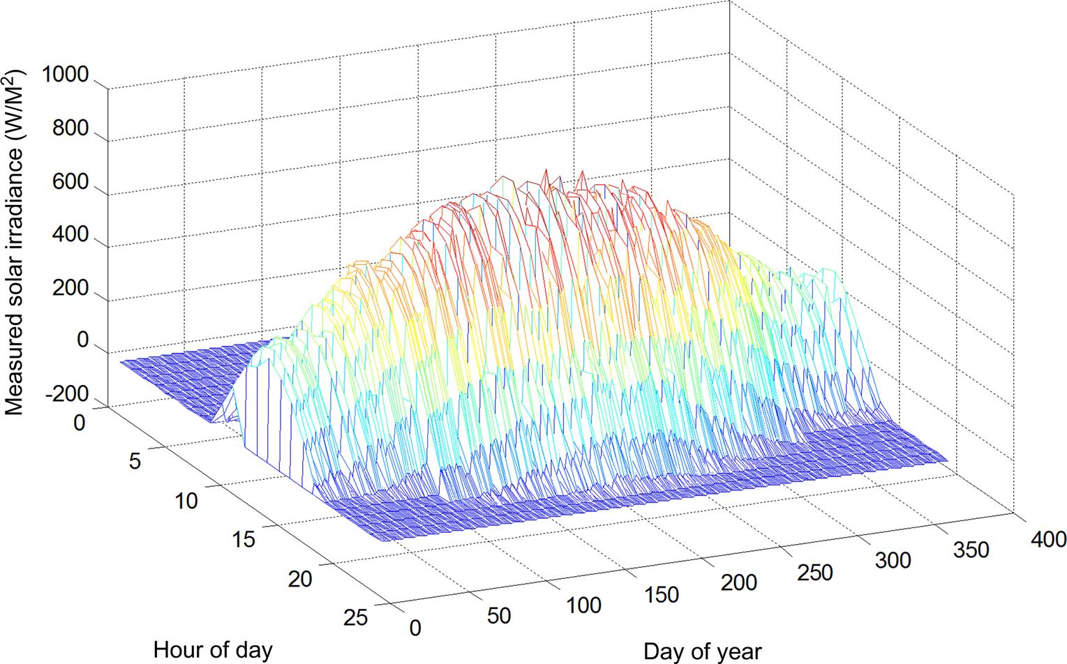
Solar irradiance is the amount of power that reaches the surface of the earth per unit area. For a given location, this amount will vary on a daily and yearly basis due to the motion of the earth relative to the sun. The amount of solar radiation also depends on the geographical location (latitude and longitude) and the climatic conditions. Cloud cover is the main factor affecting the amount of solar radiation that reaches the surface of the earth. Fig. 7.7 shows the seasonal and hourly variability in solar irradiance measured at Ames, Iowa for the year 2015.
There are a variety of models that are used to estimate the solar irradiance and PV power generation for example, the Meneil, Hottel, and Iqbal models for irradiance. Two models will be examined: The ASHRAE model [6,7] and a model developed by Tina et al. [8].
The ASHRAE model was developed by the American Society of Heating, Refrigerating, and Air Conditioning engineers to estimate the beam portion of the irradiation reaching the earth’s surface for a clear sky [6,7]. It is based on original empirical work and has the advantage that it does not depend on any atmospheric data; yet, it has been widely used in many solar applications. The direct beam radiation at sea level, ![]() , is determined by the following equation:
, is determined by the following equation:
(7.3)
where ![]() represents the apparent extraterrestrial flux,
represents the apparent extraterrestrial flux, ![]() =1140 + 75
=1140 + 75 ![]() ,
, ![]() =0.132 + 0.023
=0.132 + 0.023 ![]() is the solar zenith angle (depends on declination, latitude, and hour for a given location), and n is the day number.
is the solar zenith angle (depends on declination, latitude, and hour for a given location), and n is the day number.
Fig. 7.8 shows the maximum direct beam radiation as a function of the day of the year for latitudes ranging from 0° to 60°.

To account for the differences between the maximum solar radiation available and the actual amount reaching earth’s surface, an hourly clearness index, ![]() , has been defined as the ratio of the irradiance on a horizontal plane,
, has been defined as the ratio of the irradiance on a horizontal plane, ![]() [kW/m2] to the extraterrestrial maximum solar irradiance
[kW/m2] to the extraterrestrial maximum solar irradiance ![]() [kW/m2]:
[kW/m2]:
(7.4)
Since most PV units are installed at an angle relative to the horizontal plane, the irradiance can be modeled by an equation that accounts for this angle and the reflectivity of the ground.
(7.5)
where ![]() is the ratio of beam radiation on the tilted surface to that on a horizontal surface,
is the ratio of beam radiation on the tilted surface to that on a horizontal surface, ![]() is the fraction of the hourly radiation on the horizontal plane which is diffused, and
is the fraction of the hourly radiation on the horizontal plane which is diffused, and ![]() is the reflectance of the ground.
is the reflectance of the ground.
The power output of a PV can then be modeled using the following equation:
(7.6)
where ![]() is the surface area of the PV array (m2),
is the surface area of the PV array (m2), ![]() is the efficiency of the PV in realistic reporting conditions (RRC), and
is the efficiency of the PV in realistic reporting conditions (RRC), and ![]() is irradiance on a surface with an angle to the horizontal plane (kW/m2).
is irradiance on a surface with an angle to the horizontal plane (kW/m2).
The efficiency of a PV system will depend on a number of factors such as the temperature of the solar cell, intensity, and spectrum of the incident sunlight. The open circuit voltage is highly sensitive to changes in temperature, which could be due to variation in ambient temperature, irradiance, or wind speed at the panel site [9]. Like all electronics, PV systems have lower efficiency in the heat than the cold.
Because ![]() will vary throughout the year based on latitude, the day of the year, and the hour angle, sunset hour angle, and reflectance of the ground, the parameters T and T′ will be used to account for these variations. Thus, the expressions for the power output generated by a PV array is given by the following equation:
will vary throughout the year based on latitude, the day of the year, and the hour angle, sunset hour angle, and reflectance of the ground, the parameters T and T′ will be used to account for these variations. Thus, the expressions for the power output generated by a PV array is given by the following equation:
(7.7)
where
in which ![]() is a geometric factor, the ratio of beam radiation on the tilted surface to that of a horizontal surface at any time,
is a geometric factor, the ratio of beam radiation on the tilted surface to that of a horizontal surface at any time, ![]() is the reflectance of the ground,
is the reflectance of the ground, ![]() is the tilt angle measured in degrees,
is the tilt angle measured in degrees, ![]() is the ratio of the diffuse radiation in an hour to the diffuse radiation in a day,
is the ratio of the diffuse radiation in an hour to the diffuse radiation in a day, ![]() is the extraterrestrial radiation on a horizontal surface (
is the extraterrestrial radiation on a horizontal surface (![]() ), and
), and ![]() is the parameter in the functional form for
is the parameter in the functional form for ![]() (
(![]() ).
).
The hourly clearness index,![]() , can be considered a random variable due to weather conditions such as cloud cover and visibility factors such as mist and haze. From sampled values of
, can be considered a random variable due to weather conditions such as cloud cover and visibility factors such as mist and haze. From sampled values of ![]() over a period of time, it is possible to obtain a probability density function
over a period of time, it is possible to obtain a probability density function ![]() for
for ![]() . There are four PDFs typically used for solar radiation. In all cases, the value of
. There are four PDFs typically used for solar radiation. In all cases, the value of ![]() represents the hourly clearness index.
represents the hourly clearness index.
Normal Distribution
(7.8)
where ![]() is the mean of the distribution, and
is the mean of the distribution, and ![]() is the standard deviation of the distribution.
is the standard deviation of the distribution.
Weibull Distribution
(7.9)
where ![]() is the shape parameter of the distribution, and
is the shape parameter of the distribution, and ![]() is the scale parameter of the distribution.
is the scale parameter of the distribution.
Extreme Value Distribution
(7.10)
where ![]() is the location parameter of the distribution, and
is the location parameter of the distribution, and ![]() is the scale parameter of the distribution.
is the scale parameter of the distribution.
Beta Distribution
(7.11)
where ![]() is the first shape parameter of the distribution, and
is the first shape parameter of the distribution, and ![]() is the second shape parameter of the distribution.
is the second shape parameter of the distribution.
It has been observed that the choice of an adequate PDF model may depend on latitude [10].
7.3 Effects of DGs on Distribution Networks
Correct siting and sizing DG units is crucial when implemented within an existing distribution network. In this section, we will examine how integrating DG units may have an impact on the distribution network in terms of voltage profile, power losses, system reliability, economic and environmental cost and benefits, and voltage stability of the distribution network. We will suggest several objective functions used to model optimal siting and sizing of DG units in this section.
7.3.1 Voltage Profile
Random placement of DG units can produce many technical problems such as voltage rise, voltage fluctuations, and the introduction of harmonics and transients. When installed in a distribution network, there can be a mismatch between the reactive power requirements of the load and the reactive power supplied by the system. In weakly loaded systems, DG integration may result in high-voltage problems and interfere with standard voltage regulation practices [3]. The stochastic nature of renewable energy sources can further worsen the voltage conditions due to their intermittency and uncertainty. Intermittency can be mitigated with a combination of energy storage, spinning reserves, and demand–response management.
However, carefully siting and sizing DG units may actually lead to an improvement in the system voltage profile, which can lead to improvement in overall system performance.
One of the key objectives in choosing the size and placement of a DG unit is to minimize the voltage deviation compared to the nominal voltage (1.0 p.u.). There are several strategies that can be used to develop an objective function for the voltage profile.
One technique is to use the voltage index (![]() ) at each node in the distribution network. The location and sizing of the DG should provide the best voltage profile. The voltage deviation index is then calculated using the following equation:
) at each node in the distribution network. The location and sizing of the DG should provide the best voltage profile. The voltage deviation index is then calculated using the following equation:
(7.12)
where at bus i, a DG unit is assumed to be installed. Then, k varies from 1 to the number of all or critical buses in the system. Using Eq. (7.12), ![]() is the per-unit voltage at the kth bus and nbus is the number of buses. The optimal placement and sizing of the DG would result in the smallest value for
is the per-unit voltage at the kth bus and nbus is the number of buses. The optimal placement and sizing of the DG would result in the smallest value for ![]() [11].
[11].
Another technique is to calculate the voltage profile index (VPI) [12]. This index penalizes a size–location pair which gives higher voltage deviations from the nominal value (Vnom). The VPI is defined as follows:
(7.13)
where n is the number of buses. Using the VPI, values closer to zero indicate better network performance.
Instead of using the voltage index or VPI as objective functions, it is common to use the voltage profile as a constraint so that ![]() to ensure that it remains within acceptable operational limits.
to ensure that it remains within acceptable operational limits.
In a weakly loaded system, overvoltage problems can be mitigated by reducing the primary substation voltage, using auto transformers and voltage regulators, increasing conductor size, or shutting down DG units during light load conditions [3,13]. While day-ahead forecasts are useful for pricing within the energy market, hour-ahead forecasts are necessary for grid operators to manage and schedule spinning reserves to manage the voltage profile [4]. This poses a challenge for renewable, stochastic DG units such as wind and solar PV.
7.3.2 Power Losses
Power loss due to the resistances in overhead lines and underground cables should be minimized in the distribution network branches. The real power loss, commonly referred to as exact loss in a system is given by (7.14)–(7.16)
(7.14)
In this expression, losses are a function of the net active (P) and net reactive (Q) power injected on each bus of the network [14]. N is the number of buses. Here, the loss coefficients are defined by
(7.15)
(7.16)
where ![]() is the net real power at bus k,
is the net real power at bus k, ![]() is the net reactive power at bus k,
is the net reactive power at bus k, ![]() is the real part of the element at row i and column j of the bus impedance matrix,
is the real part of the element at row i and column j of the bus impedance matrix, ![]() is the voltage at bus k, and
is the voltage at bus k, and ![]() is the voltage angle at bus k.
is the voltage angle at bus k.
Calculating the exact power loss is computationally expensive. When developing models that include power loss, approximation formulas will often suffice. One such approximation technique is the B Matrix Power Loss Formula given by (7.17). Using the B Matrix approximation eliminates, the need to calculate the loss for each transmission line provided that the system structure remains reasonably constant [15]. This approximation works well for wide changes in the loading pattern of the system. We refer our readers to Ref. [15] for a discussion on the techniques to compute the values for the B matrix.
(7.17)
where P is the vector of all generator buses’ net real power, ![]() is the square matrix of the same dimension as P,
is the square matrix of the same dimension as P, ![]() is the vector of the same length as P, and
is the vector of the same length as P, and ![]() is a constant.
is a constant.
This can be written in terms of row and column terms given by the following equation:
(7.18)
The penetration of DG units within a network can cause significant changes in voltage magnitudes and power flows. These changes will affect power system losses. If DG units are strategically allocated, they can cause a significant reduction in losses of vulnerable feeders [16]. If a DG unit is sited near a large load, the network losses will be reduced since the load will be fed by both real and reactive power, and conversely, the network losses will increase if the generator is placed far away from the load center. When optimally sized and placed, DGs can reduce system losses by 10–20% [2].
DG technologies such as solar PV, micro turbines, and fuel cells are capable of reducing active power losses, but are incapable of delivering reactive power [2]. DG units with power electronic interfaces (depending on the inverter technology used) are capable of supplying and consuming reactive power when required. The management of the apparent power may require sophisticated control mechanisms during DG implementation [3].
7.3.3 Power Distribution System Reliability
7.3.3.1 An Introduction on Importance of Reliability Studies in Distribution Systems
Over the past 100 years, the role of electricity has evolved. In today’s information age, reliable electricity is no longer a luxury; it is now a basic requirement of many customers. It is critical to all aspects of safely operating our cities, businesses, and homes. However, the electric grids have not kept pace with surging demand. Even with substantial improvements in energy-efficient buildings, electricity demand has increased from 1500 billion kW h in 1970 to over 3700 billion kW h in 2004 and is projected to reach 5600 billion kW h by 2030 [17]. With the growing demand and increasing dependence on electricity energy, the necessity to achieve an acceptable level of reliability becomes a crucial issue for decision makers of power systems [18]. Therefore, the utilities in electricity industry have to improve systems continuously to meet customers’ reliability requirements.
Distribution systems, as the final level in delivery of electricity to the end users, have an undeniable role in providing reliable electricity to the costumers. However, the technical studies show that more than 90% of the customer service interruptions occur due to failures in different equipment of these systems [19]. This represents the importance of this sector in reliability level of customers and emphasizes on the reliability improvement of distribution systems.
Reliability is a measure of the system’s ability to meet the electricity needs of customers, which can be used as a means of assessing the past performance of a system or predicting its future. For distribution systems, at the present time, reliability evaluations are more widely used in assessing the system performance. Assessment of system performance is a valuable procedure for three important reasons.
• It establishes the chronological changes in system performance and therefore helps to identify weak areas and the need for reinforcements.
• It establishes existing indices which serve as a guide for acceptable values in future reliability assessments.
• It enables previous predictions to be compared with actual operating experience.
Reliability assessment necessitates evaluation techniques and indices to quantify current system status and compare the merits of various reinforcement schemes.
7.3.3.2 Reliability Evaluation Methods
Power system reliability evaluation methods can be divided into two categories: (1) Analytical methods, and (2) simulation methods. In addition, the reliability evaluation may be a qualitative study, in which the main factors that impact system reliability can be determined and prioritized, or a quantitative study, where the reliability is assessed through different parameters and indices defined and calculated for the system or load points [20].
Analytical techniques represent the system by a mathematical model and evaluate the reliability indices from this model using direct numerical solutions. They generally provide expectation indices in a relatively short computing time. There are several methods to analytically evaluate reliability, including fault tree analysis, failure mode, effect, and criticality analysis, Markov processes, minimum cut-set method, and network reduction method [21]. The most common evaluation techniques using a set of approximate equations are failure mode analysis and minimum cut set analysis. Analytical approaches are based on assumptions concerning the statistical distributions of failure rate and repair times. On the contrary, assumptions are frequently required in order to simplify the problem and produce an analytical model of the system. This is particularly the case when complex systems and complex operating procedures have to be modeled. The resulting analysis can therefore lose some or much of its significance. The use of simulation techniques is very important in the reliability evaluation of such situations. Simulation methods estimate the reliability indices by simulating the actual process and random behavior of the system. Monte Carlo technique is the widely used simulation method which has two different categories [21]: (1) Sequential, and (2) nonsequential.
In a nonsequential Monte Carlo simulation (MCS), the samples are taken without considering the time dependency of the states or sequence of the events in the system. Therefore, using this method, a nonchronological state of the system is determined. On the other hand, a sequential MCS can address the sequential operating conditions of the system, and may be used to include time correlated events and states such as output generation of renewable-based generating units, demand profile, and customer decisions, which is more applicable for power system reliability studies.
The MCS methods are classified based on the methods used for sampling. Three common sampling approaches in MCS are: (1) State sampling approach; (2) system state transition sampling approach; and (3) state duration sampling approach [21].
7.3.3.3 Reliability Indices
Reliability indices are used by system planners and operators as a comparative tool to improve the quality level of service to customers. Planners use these parameters to determine the requirements for capacity additions, while operators use them to ensure that the system is robust enough to withstand possible failures without catastrophic consequences.
The vast majority of reliability indices reflect faults and failures in the distribution system. These metrics are based upon the customers’ outage data and the unserved load. They describe how often electrical service are interrupted, how many customers are involved with each outage, how long the outages lasts, and how much load goes unsupplied.
Distribution reliability indices falls into two major categories, costumer-oriented and load- and energy-oriented, which both provide detailed information about the system [18].
a. System average interruption frequency index (SAIFI)
SAIFI indicates how often an average customer is subjected to sustained interruption over a predefined time interval:
(7.19)
where ![]() is the failure rate, and
is the failure rate, and ![]() is the number of customers of load point i.
is the number of customers of load point i.
b. System average interruption duration index (SAIDI)
It indicates the total duration of interruption an average customer is subjected for a predefined time interval:
(7.20)
where ![]() is the annual outage time.
is the annual outage time.
c. Customer average interruption duration index (CAIDI)
This index indicates the average time required to restore the service:
(7.21)
d. Average service availability/unavailability index (ASAI/ASUI)
ASAI specifies the fraction of time that a customer has received the power during the predefined interval of time and is vice versa for ASUI:
(7.22.a)
(7.22.b)
where 8760 is the number of hours in a calendar year.
2. Load- and energy-oriented indices
a. Energy not supplied (ENS)
ENS specifies the average energy the customer has not received in the predefined time:
(7.23)
where ![]() is the average load connected to load point i.
is the average load connected to load point i.
b. Average energy not supplied (AENS)
(7.24)
c. Average customer curtailment index (ACCI)
(7.25)
This index differs from AENS in the same way that CAIFI differs from SAIFI. It is therefore a useful index for monitoring the changes of average energy not supplied between one calendar year and another.
7.3.3.4 DGs and Electric Distribution System Reliability
Today, changing consumer needs, combined with advances in DG technologies making them more efficient and less costly, have opened new opportunities for consumers to use DGs to meet their own energy needs, as well as electric utilities to explore possibilities to meet electric system needs with distributed generation.
Implementation of DGs offers potential benefits to distribution systems. They provide an enhanced power quality, reduce peak loads, and provide ancillary services such as reactive power and voltage support. Using DGs to meet these local system needs can add up to improvements in overall electric system reliability. Therefore, DGs can be used by electric system planners and operators to improve reliability in both direct and indirect ways.
1. Direct Effects
DGs could be used directly to support local voltage levels and avoid an outage that would have otherwise occurred due to excessive voltage sag. In addition, they can add to supply diversity and thus lead to improvements in overall system adequacy. Multiple analyses have shown that a distributed network of smaller sources provides a greater level of adequacy than a centralized system with fewer large sources, reducing both the magnitude and duration of failures [22]. However, it should also be noted that a single stand-alone distributed unit without grid backup will provide a significantly lower level of adequacy.
A study of actual operating experience determines how DG units perform in the field [23]. The study results include forced outage rates, scheduled outage factors, service factors, mean time between forced outages, and mean down times for a variety of DG technologies and duty cycles. The availability factors collected during this study are summarized in Fig. 7.9. Although the sample size for the DG equipment has been smaller than that for the central station equipment, the availability of the DG is generally comparable to that of central station equipment.
Modeling DGs of varying failure and repair rates, using a Monte Carlo evaluation technique and the unserved load as a reliability measure, has showed that DG can enhance the overall capacity of the distribution system and can be used as an alternative to the substation expansion in case of expected demand growth [24].
Integration of DGs can also help the distribution system reliability by serving a portion of the load, and also enabling feeder tie operations that were previously blocked by high-load levels. A study on an actual utility system has also shown that the addition of DG on just one feeder has led to SAIDI improvements ranged from 5 to 22% in all feeders [25].
An examination of systems with mixed centralized and distributed generation shows that the potential reliability benefits depend on a mix of factors, particularly the reliability characteristics of the distributed technology, the degree of DG penetration, and the reliability characteristics of the centralized generating technologies being replaced versus those being kept [26].
2. Indirect Effects
DGs can also improve reliability in indirect ways, by reducing stress on grid components to the extent that the individual component reliability is enhanced. This way, the number of outages caused by overloaded utility equipment diminishes. For instance, during peak load situations, higher currents may lead to thermal loss-of-life in transformers and other equipment, which in turn may lead to service interruptions. These outages are usually caused by sudden equipment failures that lead to increased loads on the remaining equipment. Such overload failures account for about 10 to 30% of all outages, depending on the utility and the region. DG can be used to reduce the number of times per year when distribution equipment is used near nameplate ratings, and thus could reduce the frequency of equipment failures and subsequent outages [27].

7.3.3.5 Reliability Models of Renewable Generators
Having a reliable distribution network requires the reliability assessments of renewable generators with stochastic nature such as wind turbines, solar arrays, electric vehicles, and others. Several reliability models have been developed for wind turbines and solar generators such as Markov-based analytical models, MCS, universal generating function, homogenous Poison process, and others. A Markov model is a set of states defined by random variables where a system can transit between states. MCS technique can generate multiple scenarios and calculate the outage frequency of a system. A two-state model (ON–OFF model) is used for a system including a wind turbine/solar generator. However, for a distribution level wind/solar farm, a multistate model is used for more accurate calculations [28,29].
7.3.4 Costs and Benefits
The costs associated with implementing a DG unit is the sum of construction costs, financial costs, O&M costs, and replacement costs. Benefits include profit of power generation, reduction of emissions of pollutants, diversification of energy sources, and potential tax credits for renewable generators. Implementing DG can delay the upgrade of transmission and distribution systems.
Construction costs represent the initial capital required to construct a renewable DG source and integrate it within the existing power system. These costs include items such as the PV panels, wind turbines, land procurement, and technologies associated with the integration of the DG sources. Labor, engineering, and management costs must also be included. Usually, the investment of fixed assets comprises the majority portion of the construction costs. Financial costs, including principal and interest, are a factor in the life-cycle cost of the DG.
O&M costs can include facility management costs, regular maintenance costs, and daily inspections. These costs can be fixed and variable. For example, for PV panels, preventative maintenance might include panel cleaning (1–2 times per year), vegetation management (1–3 times per year). However, upkeep of data acquisition and monitoring systems may only need to take place on an as-needed basis. Corrective and reactive maintenance and condition-based maintenance, such as warranty enforcement and equipment replacement include some of the costs of O&M [30].
For the purpose of modeling, the objective function for costs and benefits can be approximated by the following equations [31]:
(7.26)
where the components of the model include
(7.27)
(7.28)
(7.29)
(7.30)
(7.31)
where ![]() is the generating income, T is the number of years,
is the generating income, T is the number of years, ![]() represents the i years’ average annual operating hours for the DG,
represents the i years’ average annual operating hours for the DG, ![]() is the capacity coefficient (the ratio of the average output and the rated power of the DG),
is the capacity coefficient (the ratio of the average output and the rated power of the DG), ![]() is the power produced by the DG unit,
is the power produced by the DG unit, ![]() is the network price,
is the network price, ![]() is the emission reduction benefits,
is the emission reduction benefits, ![]() represents the conventional fuel generation environmental costs,
represents the conventional fuel generation environmental costs, ![]() represents the investment costs,
represents the investment costs, ![]() represents the cost of individual equipment,
represents the cost of individual equipment, ![]() is the average cost factor of a DG fixed investment
is the average cost factor of a DG fixed investment
![]() is the annual profit, t represents the planning years,
is the annual profit, t represents the planning years, ![]() represents the O&M cost,
represents the O&M cost, ![]() is the unit power factor (PF),
is the unit power factor (PF), ![]() represents the O&M cost per unit of power (this is a function of time and increases as the facility ages), and
represents the O&M cost per unit of power (this is a function of time and increases as the facility ages), and ![]() is the residual value.
is the residual value.
7.3.5 Voltage Stability
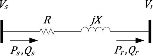
Voltage stability indices are defined as indicators to detect the voltage collapse points in a power system. They determine the reactive power loading capability of a given node of a system. A two-bus model shown in Fig. 7.10 is used to calculate the voltage stability indices. To obtain the indices, the receiving voltage is normally formulated as a function of the transferred reactive power and the conditions are satisfied which give feasible solutions for the voltage. First voltage stability index and line stability factor, two well-known voltage stability indices, are introduced in this section.
7.3.5.1 First Voltage Stability Index
Fast voltage stability index (FVSI) [32,33] determines the stable operating region of the load using the reactive power transfer. In order to obtain FVSI, we use the two-bus model (Fig. 7.10) and the following definitions:
![]() : Voltage phasor at the sending end (
: Voltage phasor at the sending end (![]() =|
=|![]() |
|![]()
![]() )
)
![]() : Voltage phasor at the receiving end (
: Voltage phasor at the receiving end (![]() =|
=|![]() |
|![]()
![]() )
)
Z, R, X: The line impedance, resistance, reactance (Z=R+jX)
(7.32)
(7.33)
Solving Eq. (7.33) for |![]() | gives:
| gives:
(7.34)
The following condition needs to be satisfied for |![]() | to have a real solution
| to have a real solution
(7.35)
Assuming ![]() ≈0, the FVSI for line sr can be defined using (7.35) as follows:
≈0, the FVSI for line sr can be defined using (7.35) as follows:
(7.36)
Based on (7.36), the system remains stable as long as FVSI is less than or equal to unity. This equation can be used to determine the maximum reactive power loading capability of a node where FVSI equals unity.
7.3.5.2 Line Stability Factor (LSF)
A similar concept applies to LSF as well [32,33]. Both active and reactive power transfer equations are used to obtain LSF. Using the two-bus model, the active and reactive powers at the receiving bus can be calculated by
(7.37.a)
(7.37.b)
when ![]() , the line losses could be neglected. Then, the active and reactive powers at the receiving end of a lossless line can be written as
, the line losses could be neglected. Then, the active and reactive powers at the receiving end of a lossless line can be written as
(7.38.a)
(7.38.b)
Since ![]() , replacing
, replacing ![]() and
and ![]() using (7.37) gives
using (7.37) gives
(7.39)
Eq. (7.38) could be written as a quadratic equation of ![]()
(7.40)
The following condition needs to be satisfied for ![]() to have a real solution:
to have a real solution:
(7.41)
As the line is assumed lossless, the sending and receiving active powers are equal (![]() ). Therefore, Eq. (7.41) can be written as
). Therefore, Eq. (7.41) can be written as
(7.42)
The line stability index (LSI) for line sr is then defined by
(7.43)
Both indices under normal and contingency conditions can be used to recognize the weakest nodes in distribution networks where there might be voltage collapse issues as the load increases. The weakest nodes in a distribution system could be the candidates for installing new DG units.
7.3.6 Fault Current
7.3.6.1 Fault Current Contribution by Upstream Grid and the DG Interface
A fundamental requirement for the connection of DG resources to the network is the total fault level which is contributed by the short circuit of the upstream grid and the DG. In medium voltage (MV) and low voltage (LV) radial networks, the fault current contribution of the upstream grid is determined by the short-circuit impedance of the HV/MV or MV/LV transformers. On the other hand, the contribution of DG sources is smaller.
DG systems have maximum acceptable fault current. The fault current level should not exceed this maximum value at every point of the distribution system. Different DG sources and their interconnection have different fault current level contributions. Three types of DG connection interfaces are synchronous generator, induction generator, and power-electronic-interfaced DG units. With DGs, the fault current levels passing through the protective device change. The amount of change in fault current level depends on the type of interface [34].
7.3.6.2 Limit Fault Current
Installing DG units increases the fault current level. Due to the increasing fault current level, protection devices such as breakers and relays that are used for normal distribution may not work for DGs. To minimize the contribution of fault current level of DG units, there are a few methods suggested such as replacing breakers and protection devices. However, these methods are costly.
One approach is to use fault current limiters (FCLs). These devices can be categorized in passive and active types. Passive FCLs are inserted permanently to the distribution system to limit fault current levels. Adding passive FCLs can cause voltage drop, lead to power loss in normal operation, and decrease the power stability of the circuit when satisfying rapidly changing demand. To avoid short coming of passive FCLs, active FCLs have low impedance during normal operation. This nonlinear impedance increases significantly during a fault condition to limit the fault current. FCLs are installed in series with synchronous-based DGs.
7.3.6.3 Calculating Fault Current
There are number of factors of a DG that contribute to the fault current level: The type of DG, the distance of DG from the fault, whether or not a transformer is placed between the fault locations, the configuration of the network between the DG and the fault, and whether we have directly connected DGs or DGs are connected via power electronics.
The fault current total impedance value ![]() is given by
is given by
(7.44)
The 3-phase fault current is given by
(7.45)
where c is the voltage factor, and ![]() is the nominal voltage of the network.
is the nominal voltage of the network.
7.3.6.4 Contribution of Upstream Grid
The contribution of the upstream grid is calculated by
(7.46)
where ![]() is the impedance of the network feeder (upstream grid) at the connection point Q, and
is the impedance of the network feeder (upstream grid) at the connection point Q, and ![]() is the impedance of the transformer.
is the impedance of the transformer. ![]() is a correction factor used for the impedance of the transformer.
is a correction factor used for the impedance of the transformer.
7.3.6.5 Contribution of DG Unit
The contribution of the DG unit is calculated by
(7.47)
where the impedance of the generator (![]() ), the transformer (
), the transformer (![]() ) (if used), the interconnection line (
) (if used), the interconnection line (![]() ) to the substation, fault impedance (
) to the substation, fault impedance (![]() ) and the reactor (
) and the reactor (![]() ) (if used) are included, all referred to the voltage at the fault location F.
) (if used) are included, all referred to the voltage at the fault location F.
7.3.7 Harmonic Distortion
Harmonic distortion can occur as nonlinear loads and sources are introduced into the network, generating harmonics of the system voltage’s fundamental frequency. DG units of the inverter-based type (such as PV) tend to have more of an impact on the system harmonic levels than synchronous-based DG units [35]. IEEE-519 places limitations on current and voltage harmonics that can cause undesirable effects on power system equipment.
In the generation of an optimization model, harmonic distortion can be considered a constraint by limiting total harmonic distortion or individual voltage harmonic distortion at each bus. Harmonic distortion could also be optimized by reducing the power loss associated with the harmonics.
7.3.7.1 Harmonic Power Flow Analysis
When modeling harmonic power flow calculations, the system can be considered as a combination of passive elements and harmonic current sources [36]. An admittance matrix is generated according to the harmonic frequency such that linear loads utilize resistance in parallel with reactance. Nonlinear loads are modeled as current sources that inject harmonic currents into the system.
The fundamental current of the nonlinear components installed at any bus with real power P and reactive power Q is modeled as
(7.48)
The hth harmonic current is then modeled as
(7.49)
where ![]() is the ratio of the hth harmonic current to its fundamental current,
is the ratio of the hth harmonic current to its fundamental current, ![]() .
.
The branch current resulting from harmonic currents occurring in the system can be calculated by
(7.50)
where ![]() are the system harmonic currents, and
are the system harmonic currents, and ![]() is the coefficient vector of harmonic currents for the branch between bus i and j at the hth harmonic order [37].
is the coefficient vector of harmonic currents for the branch between bus i and j at the hth harmonic order [37].
The coefficient vector, ![]() , is defined to record the existence of system harmonic currents that flow through the branch. The backward current sweep technique [37] is used to build the coefficient vectors. If a bus harmonic flows through the branch, then the coefficient vector will have a value of 1 in its corresponding position. The coefficient vector will only have binary values of 0 or 1. Then, the branch voltage drop resulting from the system harmonic vector can be expressed as
, is defined to record the existence of system harmonic currents that flow through the branch. The backward current sweep technique [37] is used to build the coefficient vectors. If a bus harmonic flows through the branch, then the coefficient vector will have a value of 1 in its corresponding position. The coefficient vector will only have binary values of 0 or 1. Then, the branch voltage drop resulting from the system harmonic vector can be expressed as
(7.51)