
Profile-guided development with OpenACC
Jeff Larkin NVIDIA, Santa Clara, CA, United States
Abstract
The purpose of this chapter is to introduce OpenACC programming by accelerating a real benchmark application. Readers will learn to profile the code and incrementally improve the application by adding OpenACC directives. By the end of the chapter the example application will be transformed from a serial code to one that can run in parallel on both offloaded accelerators, such as Graphic Processing Units (GPUs), and multicore targets, such as multicore Central Processing Units (CPUs).
At the end of this chapter the reader will have a basic understanding of:
• The OpenACC kernels directive
• OpenACC data directives and clauses
• The PGProf profiler
• OpenACC’s three levels of parallelism
• Data dependencies
Keywords
Parallel programming; Data dependency; Data independence; Performance analysis; Performance optimization; Kernels; Loop; Offloading
The purpose of this chapter is to introduce OpenACC programming by accelerating a real benchmark application. Readers will learn to profile the code and incrementally improve the application by adding OpenACC directives. By the end of the chapter the example application will be transformed from a serial code to one that can run in parallel on both offloaded accelerators, such as Graphic Processing Units (GPUs), and multicore targets, such as multicore Central Processing Units (CPUs).
At the end of this chapter the reader will have a basic understanding of:
• The OpenACC kernels directive
• OpenACC data directives and clauses
• The PGProf profiler
• OpenACC’s three levels of parallelism
• Data dependencies
Compiler directives, such as OpenACC, provide developers with a means of expressing information to the compiler that is above and beyond what is available in the standard programming languages. For instance, OpenACC provides mechanisms for expressing parallelism of loops and the movement of data between distinct physical memories, neither of which is directly available in C, C++, or Fortran, the base languages supported by OpenACC. As such, programmers typically add directives to existing codes incrementally, applying the directives first to high-impact functions and loops and then address other parts of the code as they becoming increasingly important. Profile-guided development is a technique that uses performance analysis tools to inform the programmer at each step which parts of the application will deliver the greatest impact once accelerated. In this chapter we will use The Portland Group (PGI) compiler and PGPROF performance analysis tool to accelerate a benchmark code through incremental improvements. By the end of this chapter we will have taken a serial benchmark and parallelized it completely with OpenACC.
Prerequisites for completing this chapter: a working OpenACC compiler and make executable (the NVIDIA OpenACC Toolkit will be used in the examples); the ability to read, understand, and compile a C or Fortran code; the ability to run the executable produced by the OpenACC compiler.
Benchmark Code: Conjugate Gradient
Throughout this chapter we will be working with a simple benchmark code that implements the conjugate gradient method. The conjugate gradient method is an iterative method to approximate the solution to a sparse system of linear equations that is too large to be solved directly. It is not necessary to understand the mathematics of this method to complete this chapter; a benchmark implementing this method has been provided in both C and Fortran. For brevity, only the C code samples will be shown in this chapter, but the steps can be applied in the same way to the Fortran version. The code used in this chapter is licensed under the Apache License, Version 2.0, please read the included license for more details.
The example code has two data structures of interest. The first is a Vector structure, which contains a pointer to an array and an integer storing the length of the array. The second structure is a Matrix, which stores a sparse 2D Matrix in compressed sparse row format, meaning that only the non-zero elements of each row are stored, along with metadata representing where the elements would reside in the full matrix if it were stored with both zero and non-zero elements. These two data structures, along with several functions for creating, destroying, and manipulating these data structures are found in vector.h and matrix.h respectively.
The first step to profile-guided development is simply to build the code and obtain a baseline profile. We’ll use this profile to inform our first steps in accelerating the code and also as a point of comparison for each successive step, both in terms of correctness and performance. A makefile has been provided with the benchmark code, which is preconfigured to build with the PGI compiler. If you are using a different OpenACC compiler, it will be necessary to modify the Makefile to use this compiler.
Building the Code
The provided makefile will build the serial code for the CPU using the PGI compiler without modification simply by running the make command. In order to obtain some additional information to help with our initial performance study, we’ll modify the compiler flags to add several profiling options.
• -Minfo=all,ccff: This compiler flag instructs the compiler to print information about how it optimizes the code and additionally embed this information in the executable for use by tools that support the common compiler feedback format.
The modified makefile is shown in Fig. 1.

At this point we have an executable (cg.x) that will serially execute the CG benchmark. The expected output is found in Fig. 2. The exact time required to run the executable will vary depending on CPU performance, but the total iterations and tolerance values should always match the values shown.

Initial Benchmarking
We will now use the PGProf profiler to obtain a baseline CPU profile for the code. This will help us to understand where the executable is spending its time so that we can focus our efforts on the functions and loops that will deliver the greatest performance speed-up. The PGProf profiler is installed with the PGI Compiler and OpenACC Toolkit. To open it, use the pgprof command from your command terminal. Once the profiler window is open, select New Session from the File menu, opening the Create New Session dialog box. By the box labeled File, press the Browse button and browse to and select your executable, which will be called cg.x. Once you have selected your executable, press the Next button and then the Finish button. At this point the profiler will run the executable, sampling the state of the program at a regular frequency to gather performance information. When complete, choose the CPU Details tab in the bottom part of the window to display a table of the most important functions in the executable. The window will look similar to what is shown in Fig. 3.

At this point, double-clicking on the most time-consuming function, matvec, will bring up a dialog to choose the location of your source files. Once you have selected the directory containing your sources, a new tab will be opened to the matvec routine in matrix_functions.h. The loop on line 33 will have a symbol in the margin to the left indicating that the profiler is able to read compiler feedback about this loop. Hovering over the graph symbol will bring up a box showing information about what optimizations the compiler was able to perform on the loop and the computational intensity of the loop. See Fig. 4 for an example.

Reading compiler feedback is the only way to understand what information the compiler is able to determine about your code and what actions it takes based on this information. The compiler may choose to rearrange the loops in your code, break them into more manageable chunks, parallelize the code to run using vector instructions such as SSE or AVX, or maybe not do anything at all because it is unable to determine what optimizations will be safe and profitable. Frequently the programmer will know information about the code that the compiler is not able to learn on its own, resulting in the compiler missing optimization and parallelization opportunities. Throughout this chapter we will be providing the compiler with more information to improve the actions it takes to optimize and parallelize this code. This is, in many ways, the primary goal of OpenACC programming: providing the compiler with enough additional information about the code that it can made good decisions on how to parallelize it to any hardware.
Exploring the CPU performance table we see that there’s three functions of interest: matvec, waxpy, and dot. The fourth most time-consuming routine is allocate_3d_poisson_matrix, which is an initialization routine that is only run once, so it will be ignored. Examining the code shows that the matvec routine contains a doubly nested loop that performance a sparse matrix/vector product and the other two routines both contain a single loop that perform two common vector operations (aX + bY and dot product). These are the three loop nests where we will focus our efforts to parallelize the benchmark.
Describe Parallelism
Now that we know where the code is spending its time, let’s begin to parallelize the important loops. It is generally a best practice to start at the top of the time-consuming routines and work your way down, since speeding up a routine that takes up 75% of the execution time will have a much greater impact on the performance of the code than speeding up one that only takes up 15%. That would mean that we should focus our effort first on the matvec routine and then move on to waxpby and dot. Since this may be your first ever OpenACC code, however, let’s start with the simplest of these three functions and work our way up to the more complex. The reason against starting with matvec will become evident shortly.
Accelerating Waxpby
On line 33 of vector_functions.h we’ll begin by parallelizing the waxpby routine. This function contains just one loop, which we will parallelize by adding the OpenACC kernels pragma immediately before the start of the loop. With this pragma added we need to inform the compiler that we are providing it with OpenACC pragmas and ask it to build the code for a target accelerator. I will be running the code on a machine that contains an NVIDIA Tesla K20c GPU, so I will choose the tesla accelerator target. Enable OpenACC for NVIDIA GPUs using the −ta=tesla command-line option. Although the compiler is targeting NVIDIA Tesla GPUs, which are intended for datacenter environments, the resulting code should run on other NVIDIA GPUs as well. The Makefile changes can be found in Fig. 5 and the compiler feedback for the waxpby routine is found in Fig. 6.


We see from the compiler feedback that although it generated a GPU kernel, something went wrong when it tried to parallelize the loop. Specifically, the compiler believes that a data dependency could exist between iterations of the loop. A data dependency occurs when one loop iteration depends upon data from another loop iteration. Close examination of the loop body reveals that each iteration of the loop is completely data-independent of each other iteration, meaning that the results calculated in one iteration will not be used by any other. So why does the compiler believe that the loop has a data dependency? The problem lies in the low-level nature of the C and C++ programming languages, which represent arrays simply as pointers into memory; pointers which can potentially point to the same memory. The problem is that the compile cannot prove that the three arrays used in the loop do not alias, or overlap, with each other, so it has to assume that parallelizing the loop would be unsafe. We can provide the compiler with more information in one of two ways. One possibility is to give the compiler more information about the pointers by promising that they will never alias. This can be done by adding the C99 restrict keyword. While this is not a C++ keyword, the PGI compiler will accept this keyword in C++ codes. 1 We could also give the compiler more information about the loop itself using the OpenACC loop directive. The loop directive gives an OpenACC compiler additional information about the very next loop. We can use the loop independent clause to inform the OpenACC compiler that all iterations of the loop are independent, meaning that no two iterations depend up the data of the other, thus overriding the compiler’s dependency analysis of the loop. Both solutions are promises that the programmer makes to the compiler about the code. If the promise is broken then unpredictable results can occur. In this code, we cannot make the guarantee that our vectors will not alias, since at times the function is called with y and w being the same vector, so we will use loop independent instead. The final code for waxpby appears in Fig. 7 along with compiler feedback in Fig. 8. Notice from the compiler feedback that the compiler has now determined that the loop at line 41 is parallelizable.


Looking more closely at the compiler feedback, notice that the compiler did more than just parallelize the loop for my GPU. The compiler understands that my target accelerator has a physically distinct memory from my host CPU, so it will be necessary to relocate my input arrays to the GPU for processing and my output array back for use later. The output for line 40 tells us that it recognizes that xcoefs and ycoefs are input arrays, so it generates a copy in to the GPU, and wcoefs is an output array, so it generates a copy out of the GPU. What the feedback is actually showing are data clauses, additional information about how the data within our compute region is used. In this case, the compiler was able to correctly determine the size, shape, and usage of our three arrays, so it generated implicit data clauses for those arrays. Sometimes the compiler will be overly cautious about data movement, so it is necessary for the programmer to override its decisions by adding explicit data clauses to the kernels directive. Other times the compiler cannot actually determine the size or shape of the arrays used within a region, so it will abort and ask for more information, as you will see when we work on the matvec routine.
Before moving on, it is always important to recompile and rerun the code to check for any errors that we may have introduced. It is much simpler to find and correct errors after making small changes than waiting until after we’ve made a lot of changes. After rerunning the code you should see that you’re still getting the same answers, but the code has now slowed down. If we rerun the executable within the PGProf profiler now, we’ll see the reason for the slowdown. Fig. 9 shows the GPU timeline that the profile gathered when I reran the executable, zoomed in a bit for clarity. What we see across the timeline are individual GPU operations (kernels) and associated data transfers. Notice that for each call to waxpby we now copy two arrays to the device and one array back for use by other function. This is really inefficient. Ideally we’ll want to leave our data in GPU memory for as long as possible and avoid these intermediate data transfers. The only way to do that is to accelerate the remaining functions so that the data transfers become unnecessary.

Accelerating Dot
Let’s quickly look at the dot routine as well, because the compiler will help us in other was when we use the OpenACC kernels pragma. Just as before, we will add a kernels pragma around the interesting loop and recompile the code. Fig. 10 shows the OpenACC version of the function and Fig. 11 shows the compiler feedback. Notice in the compiler feedback that at line 29 it generated an implicit reduction. Every iteration of the loop calculates its own value for xcoefs[i]*ycoefs[i], but the compiler recognizes that we don’t actually care about each of those results, but rather the sum of those results. A reduction takes the n distinct values that get calculated in the loop and reduces them down to the one value we care about: the sum. It is important to understand that due to the imprecise nature of floating point arithmetic a parallel reduction may result in a slightly different, but equally correct, answer than adding the numbers one at a time sequentially. How much this will vary will depend on the actual numbers being added together, how many numbers are being summed, and the order the operations happen, but the difference could be a few bits or even several digits. Remember, both the sequential and parallel sum are correct because floating point arithmetic is imprecise by its nature. Because we used the kernels pragma to parallelize this loop, the compiler handled the complexity of identifying this reduction for us. Had we used the more advanced parallel pragma instead, it would have been our responsibility to inform the compiler of the reduction. Before moving on to the next section, don’t forget to rerun the code to check for mistakes.


Accelerating Matvec
The final routine that needs to be accelerated is the matvec routine. As was said earlier, were this more than a teaching exercise this routine would have been the correct place to start our effort, since it is the most dominant routine by far, but this routine has some interesting complexities that require us to take additional steps when expressing the parallelism contained within. Let’s start by taking the same approach as the other two routines: add the restrict keyword to our arrays and wrap our loop nest with a kernels pragma. When we attempt to build this routine, however, the compiler issues an error message, as shown in Fig. 12.

The most important part of the compiler output here is the accelerator restriction at line 34, which states that it doesn’t know how to calculate the size of the arrays used inside the kernels region, specifically the three arrays used within the innermost loop. In the previous two examples, the compiler could determine based on the number of loop iterations how much data needed to be relocated to the accelerator, but because the loop bounds inside of matvec are hidden within our matrix data structure, it is impossible for the compiler to determine how to relocate the key arrays. This is a case where we will need to add explicit data clauses to our kernels pragma to give the compiler more information about our data structures. Table 1 lists the five most common data clauses and their meanings. We’ve already seen the copyin and copyout clauses implicitly used by the compiler in the previous functions.
Table 1
Data Clauses and Their Meanings
| Clause | Behavior |
| copyin | Check whether the listed variables are already present on the device, if not create space and copy the current data in to the device copy |
| copyout | Check whether the listed variables are already present on the device, if not create space on the device and copy the resulting data out of the device copy after the last use |
| copy | Behaves like the variables appeared in both a copyin and copyout data clause |
| create | Check whether the listed variables are already present on the device, if not create empty space on the device |
| present | Assume that the listed variables are already present on the device |
In order for the compiler to parallelize the loop nest in matvec for my GPU, which requires the offloading of data, we’ll need to tell the compiler the shape of at least the three arrays used within the inner loop. All three of these arrays are used only for reading, so we can use a copyin data clause, but we’ll need to tell the compiler the shape of the arrays, which we can learn by looking at how they are allocated in the allocate_3d_poisson_matrix function, located in matrix.h. The data clauses accept a list of variables with information about the size and shape of the variables. In C and C++ the size and shape of the arrays are provided using square brackets ([ and ]) containing the starting index and number of elements to transfer, e.g., [0:100] to start copying at index 0 and copy 100 elements of the array. In Fortran the syntax uses parentheses and used the first and last index to copy, for instance (1:100) to start at index 1 and copy all elements up to element 100 in the array. The difference in syntax between these programming languages is intentional to fit with the conventions of the base programming languages. Since Fortran variables are self-describing, the size and shape information can be left off if the entire variable needs to be moved to the device.
Fig. 13 shows the modified code for the matvec function. Notice the addition of a copy data clause to the kernels direction, which informs the compiler both how to allocate space for the affected variables on the accelerator, but also that the data is only needed as input to the loops. With this change, we’re now able to run the full CG calculation in parallel on the accelerator and get correct answers, but notice in Fig. 14 that the runtime is now longer than our original code.


Let’s rerun the executable using the PGProf profiler to see if we can determine why the code is so much slower than it was before, even though it is now running in parallel on our GPU. Fig. 15 shows the GPU timeline returned from PGProf, zoomed in for clarity.

Describe Data Movement
In order to ensure that our three accelerated routines share the device arrays and remove the necessity to copy data to and from the device in each function, we will introduce OpenACC data directives to express the desired data motion at a higher level in the program call tree. By taking control of the data motion from the compiler we are able to express our knowledge about how the data is actually used by the program as a whole, rather than requiring the compiler to make cautious decisions based only on how the data is used inside individual functions.
OpenACC has two different types of directives for managing the allocation of device memory: structured and unstructured. The structured approach has a defined beginning and end within the same program scope, for instance a function, which limits its ability to express data motion to programs where the data motion can be neatly represented in a structured way. Unstructured data directives provide the programmer more flexibility in where data management occurs, allowing the allocation and deletion of device data to happen in different places in the program. While this is especially useful in C++ classes, where data is frequently allocated in a constructor and deleted in the destructor, it also provides the programmer with a clean way to manage the device memory alongside of the management of host memory. For this reason we’ll use the unstructured data directives to manage the device data in the existing data management routines.
The enter data and exit data directives are used for unstructured data management. As the names imply, enter data specifies the beginning of a variable’s lifetime on the device, which are controlled by the create or copyin data clause. Similarly the exit data directive marks the end of the lifetime of a variable with the copyout, release, and delete data clauses. Since data is passed between functions, it is actually possible that the same variable may have multiple enter and exit data directives that refer to it, so the runtime will keep a count of how many times a variable has been referenced, ensuring that the data isn’t removed from the device until it is no longer needed on the device. The runtime will also use this reference count to determine whether it is necessary to copy data to or from the device, which only occurs on the first and last references to the data if needed. Table 2 expands upon Table 1 adding the two data clauses that may only appear on exit data directives.
Table 2
Additional Data Clauses Only Valid on Exit Data Directives
| Clause | Behavior |
| delete | Listed variables will be immediately removed from the device, regardless of reference count, without triggering any data copy |
| release | The reference count for listed variables will be reduced. If the reference count reaches 0, the variable will be removed from the device without triggering any data copy |
Describing Data Movement of Matrix and Vector
To avoid unnecessary data movement in each of the three functions we’ve parallelized we will add unstructured data directives to the functions that manage the data in our Matrix and Vector structures. It is important to remember that OpenACC’s data model is host-first, meaning that data directives that allocate data on the device must appear after host allocations (malloc, allocate, new, etc.) and data directives that deallocate device data must appear before host deallocations (free, deallocate, delete, etc.). Given this, let’s add enter data directives to the allocate_3d_poisson_matrix and allocate_vector functions, in matrix.h and vector.h respectively. Since allocate_3d_poisson_matrix does some additional initialization, it is simplest to add the directives to the end of the routine so that the device copy of the data structure will contain the initialized data.
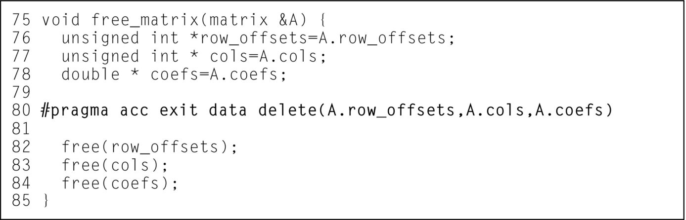
Fig. 16 shows an abbreviated listing of the allocate_3d_poisson_matrix function with the enter data directives added. It may seem strange at first to copy A to the device and then all of the member arrays inside A. The A structure contains two scalar numbers, plus 3 pointers that are used on the device. The copyin of A at line 71 copies the structure, with the 5 elements that I just described. When the 3 pointers are copied, however, they will contain pointers back to the host memory, since the pointers were simply copied to the device. It is then necessary to copy the data pointed to by those pointers, which is what the pragma at line 72 achieves. Line 72 gives the three arrays contained in A shapes and copies their data to the device. When removing the data from the device in the free_matrix function, these operations should be done in the reverse order, as shown in Fig. 17.

The allocate_vector and free_vector functions can be similarly modified to relocate Vector structures to the accelerator as well. Since allocate_vector does not initialize the vector with any data, the create data clause can be used to allocate space without causing any data copies to occur, as shown in Fig. 18.

At this point the benchmark will run with all Matrix and Vector data structures residing on the device for the entire calculation, but it will give incorrect results because the code fails to initialize the vector data structures on the accelerator. To fix this, it is necessary to modify the initialize_vector function to update the device data with the initialized host data. This can be done with the OpenACC update directive. The update directive causes the data in the host and device copies of a variable to be made consistent, either by copying the data from the device copy to the host, or vice versa. On architectures with a unified memory for both the host and accelerator devices update operations are ignored.
The update directive accepts a device or self clause to declare which copy of the data should be modified. Since we want to update the device’s data using the data from the host, the device clause is used, specifying that the device’s copy of the coefficients array should updated. An update directive can be used in the initialize_vector function to copy the data in the initialized host vector to the device, as shown in Fig. 19. When using the update directive, the amount of data to update is specified in the same way as the data clauses, as shown earlier. In the case of Fortran arrays, if the entire array needs to be updated then the bounds can be left off.

One point of confusion for new OpenACC programmers is why the clause for updating the host’s arrays is called self. OpenACC 1.0 used the host keyword to specify that the host array should be updated with the data from the device array, but since OpenACC 2.0 opened up the possibility of nesting OpenACC regions within other OpenACC compute regions, it is possible that the thread performing the update isn’t on the host, but rather is on a different accelerator. Fig. 20 shows a pseudo-code example of a kernels region nested within another kernels region. When the update on line 4 occurs, the device running the outer kernels region will copy the values from its copy of A to the device that will run the kernels region on line 5. At line 8 the device running the outer kernels region needs to copy back the results from the inner region. Saying update the host copy is not correct, since the kernels region at line 1 might not be running on the host, so OpenACC 2.0 introduced the idea of update self, as-in update my copy of the data with the device data. The host keyword still exists in OpenACC 2.0 and beyond, but it has been defined to always mean self instead.

At this point building and running the benchmark code results in a large performance improvement on the example system. Examining the PGProf timeline (Fig. 21) shows that the data is copied to the device at the very beginning of the execution and only the resulting norm is copied back periodically. This is because we’ve expressed to the compiler that it should generate our data structures directly on the accelerator and the compute regions that were added in the previous section check for the presence of the data and, upon finding the data on the device, reuse the existing device data. On accelerators with discrete memory, such as the GPU used in this example, expressing data motion is often the step where programmers will see the greatest speed-up, since the significant bottleneck of copying data over the PCIe bus is removed. It is tempting to think that because this step creates such a large speed-up it should be done first. Doing so is often error prone, however, since it would be necessary to introduce update directives each time an unaccelerated loop is encountered. It is simpler instead to first put all of the loops on the device, at least within a significant portion of the code, and then eliminate unnecessary data transfers. Forgetting to eliminate an unneeded data transfer is simply a performance bug, which is simple to identify with the profiler, while forgetting an update directive because data directives were added to the program too soon is a correctness bug that is often much more difficult to find.

Optimize Loops
At this point the benchmark code is now running 2× faster than the original serial code on the testbed machine, but is this the fastest the code can be? Up to this point all of the pragmas we’ve added to the code should improve the performance of the benchmark on any parallel processor, but to achieve the best performance on the testbed machine, we’ll need to start applying target-specific optimizations. Fortunately OpenACC provides a means for specifying a device_type for optimizations so that the additional clauses will only apply when built for the specified device type. Let’s start by accessing the compiler feedback from the current code, particularly the matvec routine, which is our most time-consuming routine (Fig. 22).

The compiler is providing information about how it is parallelizing the two matvec loops at lines 30 and 24, but in order to understand what it is telling us, we need to understand OpenACC’s three levels of parallelism: gangs, workers, and vectors. Starting at the bottom of the levels, vector parallelism is very tight-grained parallelism where multiple data elements are operated on with the same instruction. For instance, if I have two arrays of numbers that need to be added together, some hardware has special instructions that are able to operate on groups of numbers from each array and add them all together at the same time. How many numbers get added together by the same instruction is referred to as the vector length, and varies from machine to machine. At the top of the levels of parallelism are gangs. Gangs operate completely independently of each other, with no opportunity to synchronize with each other and no guarantees about when each gang will run in relation to other gangs. Because gang parallelism is very coarse-grained, it is very scalable. Worker parallelism falls in between gang and vector. A gang is comprised of one or more workers, each of which operate on a vector. The workers within a vector have the ability to synchronize and may share a common cache of very fast memory. Every loop parallelized by an OpenACC compiler will be mapped to at least one of these levels of parallelism, or it will be run sequentially (abbreviated seq). Fig. 23 shows the three levels of OpenACC parallelism.

With that background, we can see how the OpenACC compiler has mapped our two loops to the levels of parallelism. It has mapped the loop at line 30 to gang and vector parallelism, implicitly creating just one worker per gang, and assigned a vector length of 128. The loop at line 34 is run sequentially. Given this information we can now begin to give the compiler additional information to guide how it maps the loops to the levels of parallelism.
Reduce Vector Length
Since I’m running this benchmark on an NVIDIA GPU, I’ll use my understanding of NVIDIA GPUs and the application to make better decisions about how to parallelize the loop. For instance, I know that NVIDIA GPUs perform best when the vector loop accesses data in a stride-1 manner, meaning each successive loop iteration accesses a successive array element. Although the outer loop accesses the row_offsets array stride-1, the inner loop accesses the Acols, Acoefs, and xcoefs arrays in stride-1, making it a better target for vectorization. Adding a loop pragma above the inner loop allows us to specify what level of parallelism to use on that loop. Additionally we can specify the vector length that should be used. The compiler appears to prefer vector lengths of 128, but our inner loop always operates on 27 non-zero elements, which results in wasting 101 vector lanes each time we operate on that loop. It’d be better to reduce the vector length, given what we know about the loop count, to reduce wasted resources. Ideally we’d just reduce the vector length to 27, since we know this is the exact number of loop iterations, but this NVIDIA GPU has a hardware vector length, referred to by NVIDIA as the warp size, of 32, so let’s reduce the vector length to 32, thus wasting only 5 vector lanes rather than 101. Fig. 24 shows the matvec loops with the inner loop mapped to vector parallelism and a vector length of 32. Notice the device_type clause on the loop directive. This clause specifies that the clauses I list are only applied to the nvidia device type, meaning that they won’t affect the compiler’s decision making on other platforms.

As we see from the output in Fig. 25, this change actually negatively affected the overall performance. It is tempting to reverse this change to the code, since it didn’t help our runtime, but I feel quite confident that the decision to vectorize the innermost loop is the right decision, so instead I will turn to the profiler to better understand why I didn’t get the speed-up I expected.

Increase Parallelism
In order to determine why customizing the vector length didn’t have the desired effect, we’ll use the PGProf guided analysis mode to help determine the performance limiter. Guided analysis should be enabled by default, so after starting a new session with the current executable, select the Analysis tab and follow the suggestions provided. The analysis should eventually point toward GPU occupancy as the limiting factor, as shown in Fig. 26. Occupancy is a term used by NVIDIA to describe how well the GPU is saturated compared to how much work it could theoretically run. NVIDIA GPUs are comprised of 1 or more streaming multiprocessors, commonly referred to as SMs. An SM can manage up to 2048 concurrent threads, although not all of these threads will be actively running at the same time. The profiler output is showing that of the possible 2048 active threads, the SM only has 512 threads, resulting in 25% occupancy. The red line in Fig. 26 shows why this is: the SM can manage at most 16 threadblocks, which equate to OpenACC gangs, but it would require 64 to achieve full occupancy due to the size of the gang, which we can see from the “Threads/Block” line only has 32 threads. What all of this is showing is that by reducing the vector length to 32, the total threads per GPU threadblock is reduced to 32 too, so we need to introduce more parallelism in order to better fill the GPU.

We can increase the parallelism within the gang in one of two ways: increase the vector length or increase the workers. We know from the previous section that increasing the vector length doesn’t make any sense, since there’s not enough work in the inner loop to support a longer vector length, so we’ll try increasing the number of workers. The total work within the GPU threadblock can be thought of as the number of workers × the vector length, so the most workers we could use is 32, because 32 × 32 = 1024 GPU threads. Fig. 27 shows the final matvec loop code and Fig. 28 shows the speed-up from changing the number of workers within each gang.


On this particular test system 8 workers of 32 threads appears to be the optimal gang size. Since the device_type clause is used, these optimizations will only apply when building for NVIDIA GPUs, leaving other accelerators unaffected.
Running in Parallel on Multicore
It’s important to understand that although an NVIDIA GPU was used in this chapter, OpenACC is not a GPU programming model, but rather a general model for parallel programming. Although the loop optimizations we applied in the Optimize Loops section apply only to the GPU on which the code was running, the description of parallelism and data motion are applicable to any parallel architecture. The PGI compiler used throughout this section supports multiple accelerator targets, including GPUs from NVIDIA and AMD and multicore ×86 CPUs. So what happens if we take the code we’ve written and rerun it on a multicore CPU? Let’s start by rebuilding the code for the multicore target, instead of the tesla target (Figs. 29 and 30).


If we now run the resulting executable it will parallelize the loops on the CPU cores of the benchmark machine, rather than the GPU. It is possible to adjust the number of CPU cores used by setting the ACC_NUM_CORES environment variable to the number of CPU cores to use. Fig. 31 shows the speed-up from adjusting the number of cores from 1 to 12, the maximum number of cores on the benchmark machine. The performance plateau beyond 4 CPU cores is due to the benchmark performance becoming limited by the available CPU bandwidth.

Summary
OpenACC is a descriptive model for parallel programming and in this chapter we used several OpenACC features to describe the parallelism and data use of a benchmark application and then optimized it for a particular platform. Although the Portland Group compiler and PGProf profiler were used in this chapter, the same process could be applied to any application using a variety of OpenACC-aware tools.
1. Obtain a profile of the application to identify unexploited parallelism in the code.
2. Incrementally describe the available parallelism to the compiler. When performing this step on architectures with distinct host and accelerator memories, it is common for the code to slow down during this step.
3. Describe the data motion of the application. Compilers must always be cautious with data movement to ensure correctness, but developers are able to see the bigger picture and understand how data is shared between OpenACC regions in different functions. After describing the data and data motion to the compiler, performance will improve significantly on architectures with distinct memories.
4. Finally, use your knowledge of the application and target architecture to optimize the loops. Frequently loop optimizations will provide only small performance gains, but it is sometimes possible to give the compiler more information about the loop than it would see otherwise to obtain even larger performance gains.
Fig. 32 shows the final performance at each step in terms of speed-up over the original serial code. Notice that the final code achieves a 4× speed-up over the original, serial code, and the multicore version achieves nearly 2.5×. Although the code did slow down at times during the process, it is easy to see why particular steps resulted in a slowdown and make corrections to further improve performance. The final result of this process is a code that has can be run on a variety of parallel architectures and has been tuned for one in particular, without negatively affecting the performance of others. This is OpenACC programming in a nutshell, providing the compiler with sufficient information to run effectively on any modern machine.
