Using OpenACC for stencil and Feldkamp algorithms
Sunita Chandrasekaran*; Rengan Xu
†
; Barbara Chapman
‡
* Computer and Information Sciences, University of Delaware, Newark, DE, United States
† University of Houston, Houston, TX, United States
‡ Stony Brook University, Stony Brook, NY, United States
Abstract
This chapter shows how a directive-based model can make it possible for application scientists to “keep” their codes, accelerate them with reduced programming effort, and achieve performance equal to or better than that obtained using hand-written code and low-level programming interfaces. Specifically, this chapter covers programmers’ experiences porting two commonly used algorithms—Feldkamp and stencil—on single and multiple GPUs along with multicore platforms. These algorithms are representative of computational patterns used in a variety of domains including computational fluid dynamics, PDE solvers, MRI imaging, and image processing for computed tomography among several others. Additional discussion explains how OpenMP, another widely utilized directive-based programming model, can co-exist with OpenACC thus creating a hybrid programming strategy to target and distribute the workload across multiple GPUs.
At the end of this chapter the reader will have a basic understanding of:
• How to profile and gain a basic understanding of code characteristics for GPUs
• How to compile an OpenACC code using relevant compilation flags and analyze the compilation information
• How to incrementally improve an OpenACC code
• How to use OpenMP with OpenACC in the same code
• How to tune OpenACC code and provide relevant hints to achieve close to, or better performance than CUDA code
Keywords
OpenACC; MultiGPU; OpenMP; Stencil; Computed tomography; Parallelization; Accelerators; Compiler optimizations; Multicore; Parallel programming
This chapter shows how a directive-based model can make it possible for application scientists to “keep” their codes, accelerate them with reduced programming effort, and achieve performance equal to or better than that obtained using hand-written code and low-level programming interfaces. Specifically, this chapter covers programmers’ experiences porting two commonly used algorithms—Feldkamp and stencil—on single and multiple GPUs along with multicore platforms. These algorithms are representative of computational patterns used in a variety of domains including computational fluid dynamics, PDE solvers, MRI imaging, and image processing for computed tomography among several others. Additional discussion explains how OpenMP, another widely utilized directive-based programming model, can co-exist with OpenACC thus creating a hybrid programming strategy to target and distribute the workload across multiple GPUs.
At the end of this chapter the reader will have a basic understanding of:
• How to profile and gain a basic understanding of code characteristics for GPUs
• How to compile an OpenACC code using relevant compilation flags and analyze the compilation information
• How to incrementally improve an OpenACC code
• How to use OpenMP with OpenACC in the same code
• How to tune OpenACC code and provide relevant hints to achieve close to, or better performance than CUDA code
Introduction
Accelerators have gone mainstream in High Performance Computing (HPC), where they are being widely used in fields such as bioinformatics, molecular dynamics, computational finance, computational fluid dynamics, weather, and climate. Their power efficient, high compute capacity enables many applications to run faster and more efficiently than on general-purpose Central Processing Units (CPUs). As a result, Graphics Processing Unit (GPU) accelerators are inherently appealing for scientific applications. However, in the past GPU programming has required the use of low-level languages such as OpenCL, CUDA, and other vendor-specific interfaces. These low-level programming models imply a steep learning curve and also demand excellent programming skills; moreover, they are time consuming to write and debug. OpenACC, a directive-based high-level model addresses these programming challenges for GPUs and simplifies the porting of scientific applications to GPUs whilst not unduly sacrificing performance.
In this chapter, we discuss experiences gained while porting two algorithms to single and multiple GPUs using OpenACC. We also demonstrate how OpenACC can be used to run on multicore platforms, thus maintaining a single code base. From our experimental analysis, we conclude that efficient implementations of high-level directive-based models plus user-guided optimizations can lead to performance close to that of hand-written CUDA code.
Experimental Setup
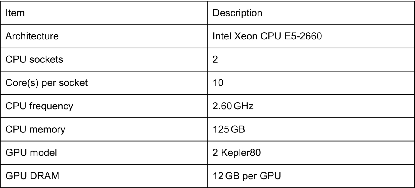
The platform used for these experiments is a multicore server containing two NVIDIA Kepler80 GPUs (see Fig. 1 for configuration details). The most recent compiler versions are used for the experiments discussed in this chapter. PGI 16.4 with the compilation flag -fast is employed to translate the CPU and OpenACC versions of the programs. CUDA 7.5 is used to compile all CUDA programs. Wall-clock time is the basis for our evaluation: results of running CPU, OpenACC, and CUDA versions of the codes are collected and compared.
Feldkamp-Davis-Kress Algorithm
Computerized Tomography (CT) is widely used in the medical sector to produce tomographic images of specific areas of the body. Succinctly, CT reconstructs an image of the original three-dimensional (3D) object from a large series of two-dimensional (2D) X-ray images. As a set of rays pass through an object around a single axis of rotation, the produced projection data is captured by an array of detectors, from which a filtered back-projection method based on the Fourier slice theorem is typically used to reconstruct the original object. Among various filtered back-projection algorithms, the Feldkamp-Davis-Kress (FDK) algorithm is mathematically straightforward and easy to implement. It is important that the image reconstructed from the acquired data be accurate. The goal of this work is to accelerate the reconstruction using directive-based programming models.
Fig. 2 shows pseudo-code for the FDK algorithm, which is comprised of three main steps:
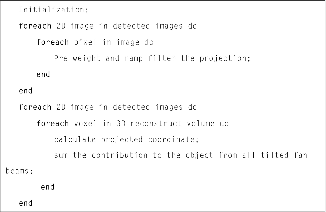
1. Weighting—calculate the projected data.
2. Filtering—filter the weighted projection by multiplying their Fourier transforms.
3. Back-projection—back-project the filtered projection over the 3D reconstruction mesh.
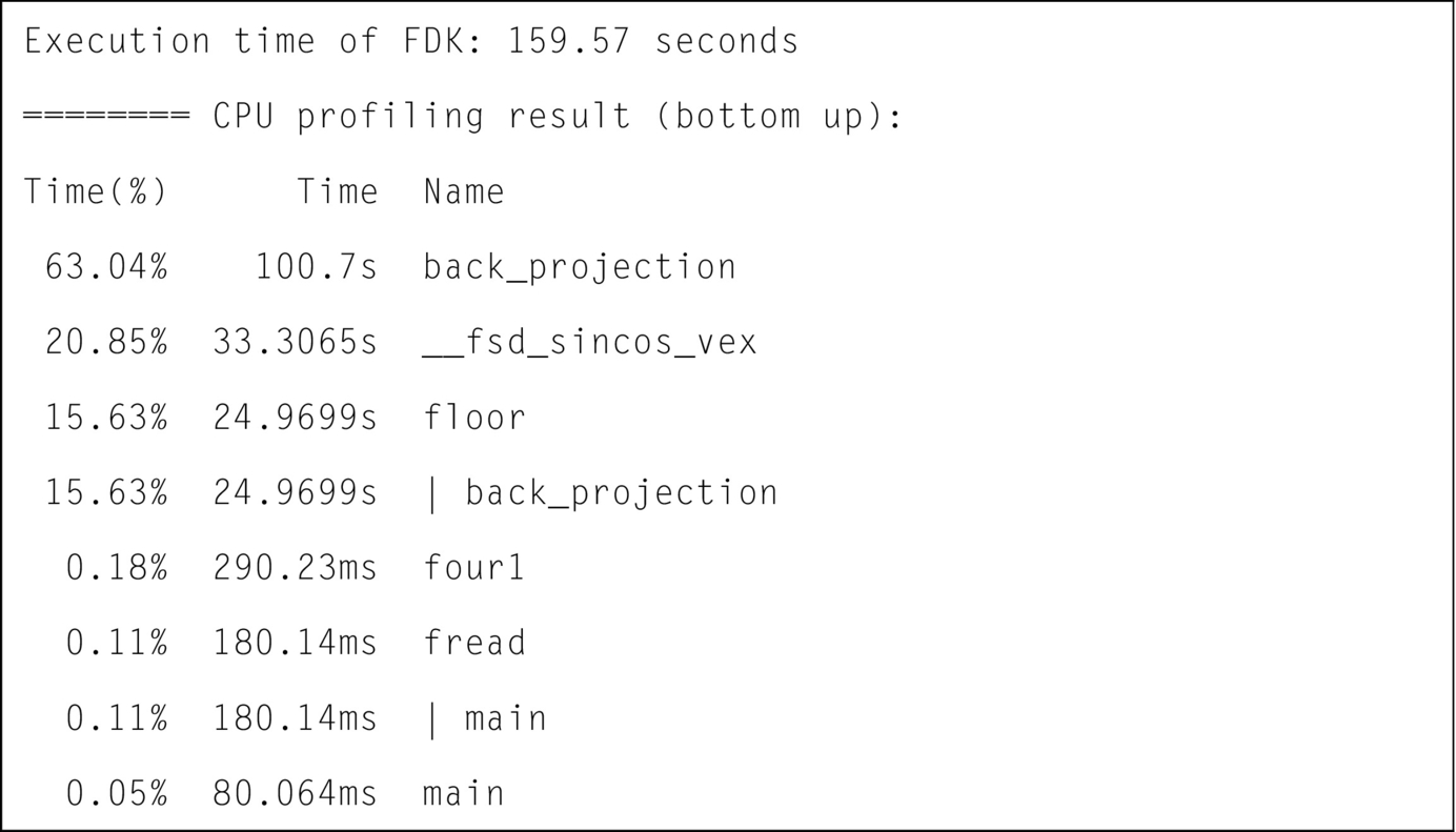
The reconstruction algorithm is computationally intensive and it has biquadratic complexity (O(N4)), where N is the number of detector pixels in one dimension. The most time-consuming step of this algorithm is back-projection. As shown in Fig. 3, a profiled example of the application shows the back-projection routines in the application accounts for nearly all the runtime (63.04% + 20.85% + 15.63% = 99.52% of the whole application). So the focus of our work is to parallelize the back-projection step.
For implementation purposes we follow the steps given by Kak and Slaney (1988). As shown in Fig. 4A, the back-projection algorithm has four loops. The three outermost loops traverse each dimension of the output 3D object, and the innermost loop accesses each of the 2D detected image slices.
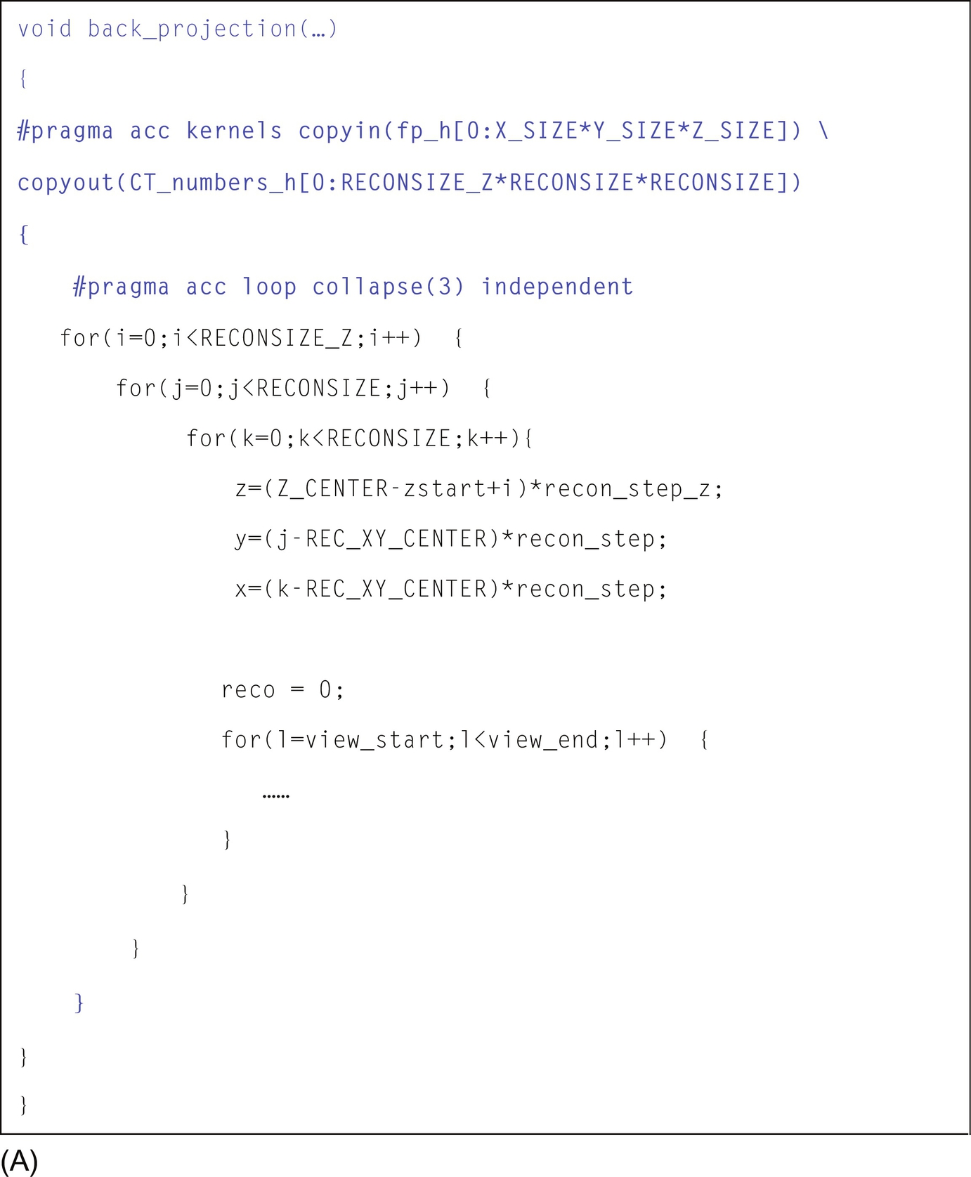
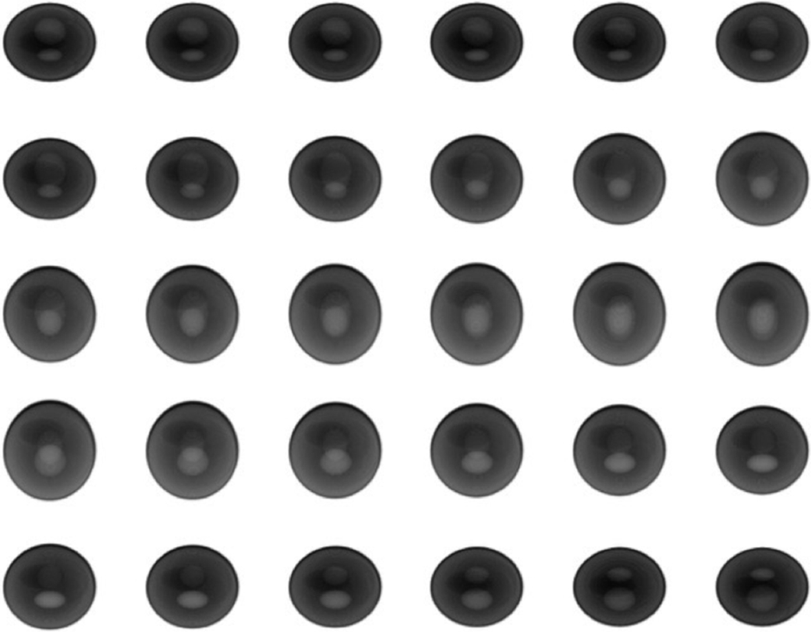
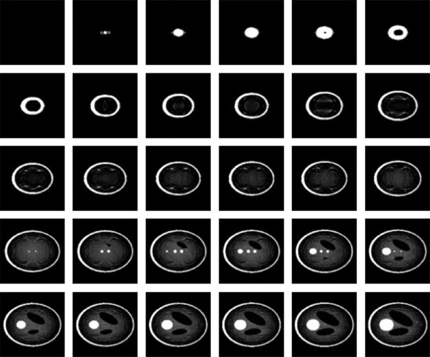
The code is first restructured so that the three outermost loops are tightly nested, and then the collapse clause from OpenACC is applied. This means that every thread sequentially executes the innermost loop. All detected images are transferred from the CPU to the GPU by using the copyin clause, and the output 3D object (i.e., many 2D image slices) is copied from GPU to CPU using the copyout clause. The implementations are evaluated using 3D Logan and Shepp (1975) head phantom data that has 300 detected images and the resolution of each image is 200 × 200. The algorithm produces a 200 × 200 × 200 reconstructed cube. The input and output images are shown towards the end of this section.
Note that results for this application are sensitive to floating-point operation ordering and precision. Hence the floating-point values of the final output on a GPU can differ from the values computed on the CPU. One reason for this is the fused multiply add (FMA) operation Pullan (2009), where the computation rn(X * Y + Z) is carried out in a single step and is only rounded once. Without FMA, rn(rn(X * Y) + Z) is composed of two steps and rounded twice. Thus, using FMA will cause the results to differ slightly; but this does not mean that the FMA implementation is incorrect. The difference in results obtained with and without FMA, respectively, may matter for certain types of codes and not for others. In our case, the observed differences (with and without FMA) were minute. However, if a complex code, e.g., a weather modeling code is under consideration, even minute differences may not be tolerable.
To compile the C version of the FDK algorithm, the following command is used (Fig. 5):

The flag “-ta=tesla” tells the compiler to generate code for the Tesla GPU. We use the option “cc35” to specify the compute capability of the targeted Tesla GPU since the Tesla GPU product family has evolved over time and now contains several generations of devices that differ with respect to their compute capabilities. The flag “nofma” tells the compiler to disable the FMA operation. The flag “-Minfo=accel” tells the compiler to output information when it translates the OpenACC code to GPU code, including information about loop scheduling, data movement, and data synchronization, and more.
In this way various implementation techniques can be explored even in the face of accuracy and precision differences.
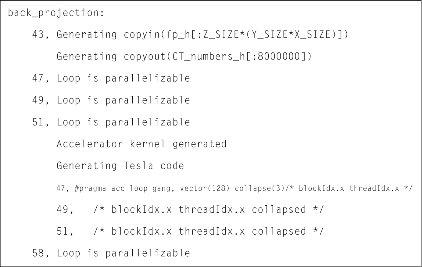
The following is the information output by the PGI compiler (Fig. 6):
OpenACC is a model that targets different accelerator architectures. In order to use it for multicore architectures, the following command is required (Fig. 7):

This command differs from the previous compiler command-line in the flags specified: –ta=multicore replaces–ta=tesla. On multicore platforms, a specification of the compute capability is not needed.
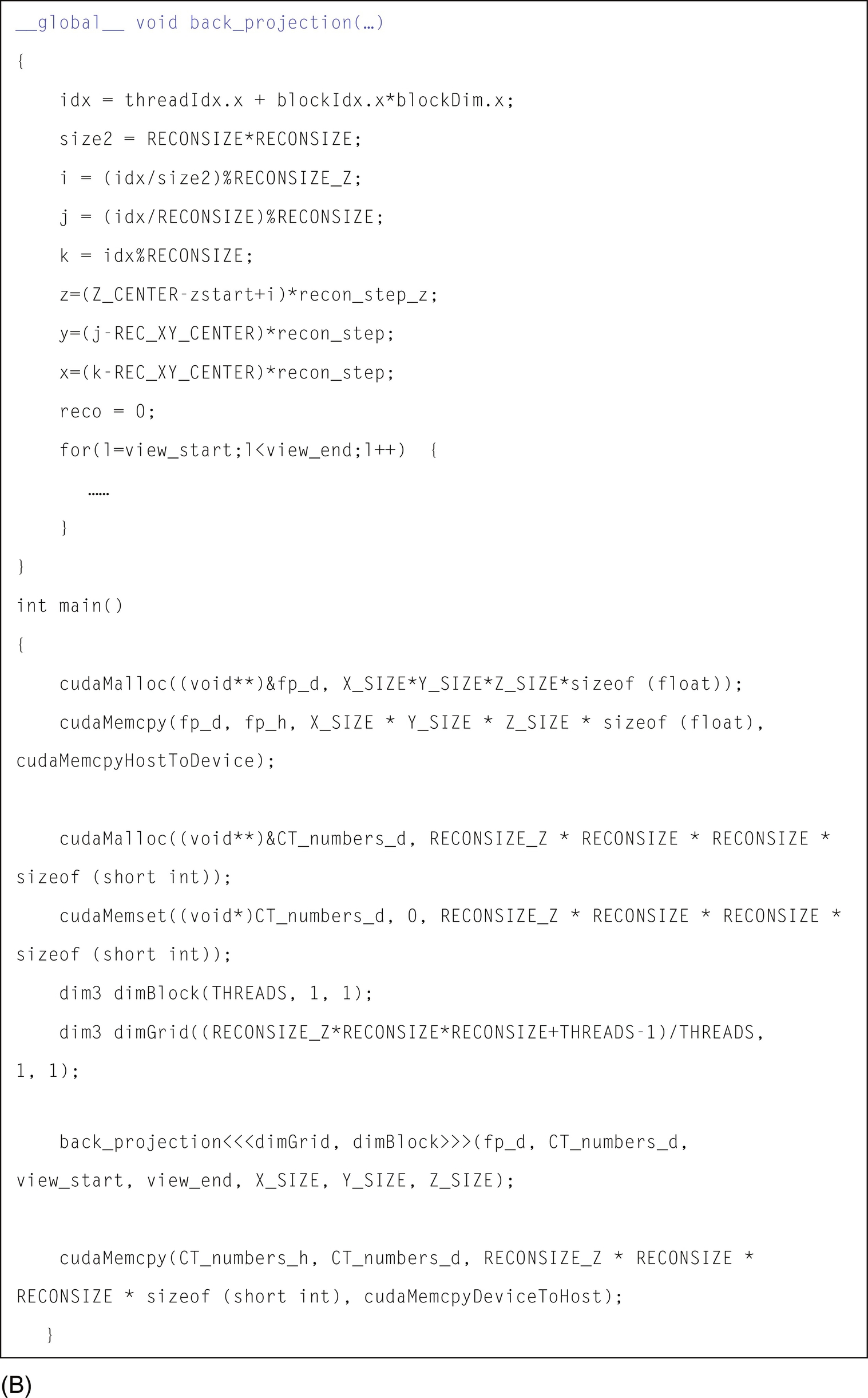
Our evaluation includes comparisons among sequential CPU versions, OpenACC versions targeting both multicore and GPUs as well as CUDA versions. The CUDA version was developed manually and the code snippet of back-projection kernel is shown in Fig. 4B.
In the OpenACC version, the three outer loops were collapsed. To keep the comparisons fair, a similar loop scheduling strategy is retained for the CUDA kernels. There are many loop schedules that can be applied by the compiler. The reader is directed to Tian et al. (2016) for more details on using different loop schedule options.
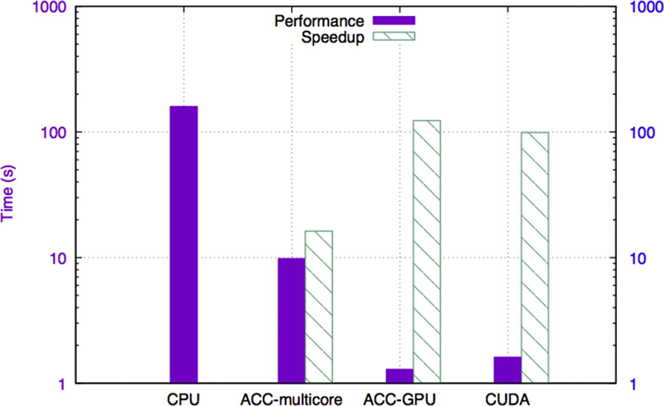
Fig. 8 shows the performance and speedup using different programming models/languages. Compared to the sequential version, the OpenACC multicore, OpenACC GPU, and CUDA versions achieved a speedup of 16.24 ×, 123.47 ×, and 98.93 ×, respectively. The performance of the OpenACC version is slightly better than that of the CUDA code. A probable reason for this is that the OpenACC compiler applied better optimizations while translating OpenACC kernels to CUDA than were implemented in the manually written CUDA kernel.
Matlab can be used to view both the input and the output images. For instance, if the resolution of the output 3D image is 200 × 200, the following Matlab script can be used to view the 180th 2D image slice in the output image (Fig. 9).
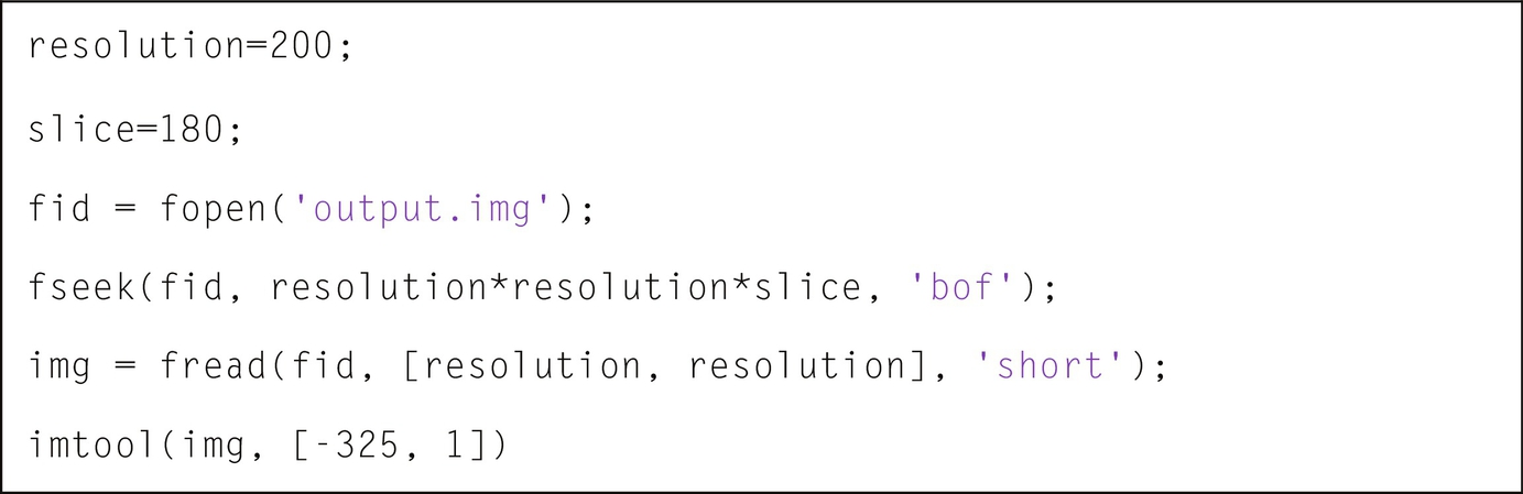
The input and output data of the 2D images are shown in Figs. 10 and 11.
2D Heat Equation
Our 2D heat equation application is a stencil-based algorithm with a high computation/communication ratio for which the workload can be distributed across several threads. The implementation uses the GPU’s global memory and obtains good performance, but it could be further improved by using GPU shared memory.
The formula to represent 2D heat conduction is explained in Whitehead & Fit-Florea (2011) and is given in Fig. 12:
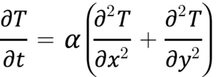
where T is temperature, t is time, α is the thermal diffusivity, and x and y are points in a grid. To solve this problem, one possible finite difference approximation is given in Fig. 13:
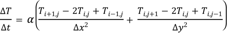
where ∆T is the temperature change over time ∆t and i, j are indices in a grid.
At program startup, a grid is set up that has boundary points with an initial temperature and inner points for which the temperature must be incrementally updated. Each inner point updates its temperature by using the previous temperature of its neighboring points and itself. The updating step diffuses the temperature from the boundary points through the grid, but it can only progress one grid point per iteration; this means that a large number of iterations can be required to reach a steady temperature state across all points in the grid.
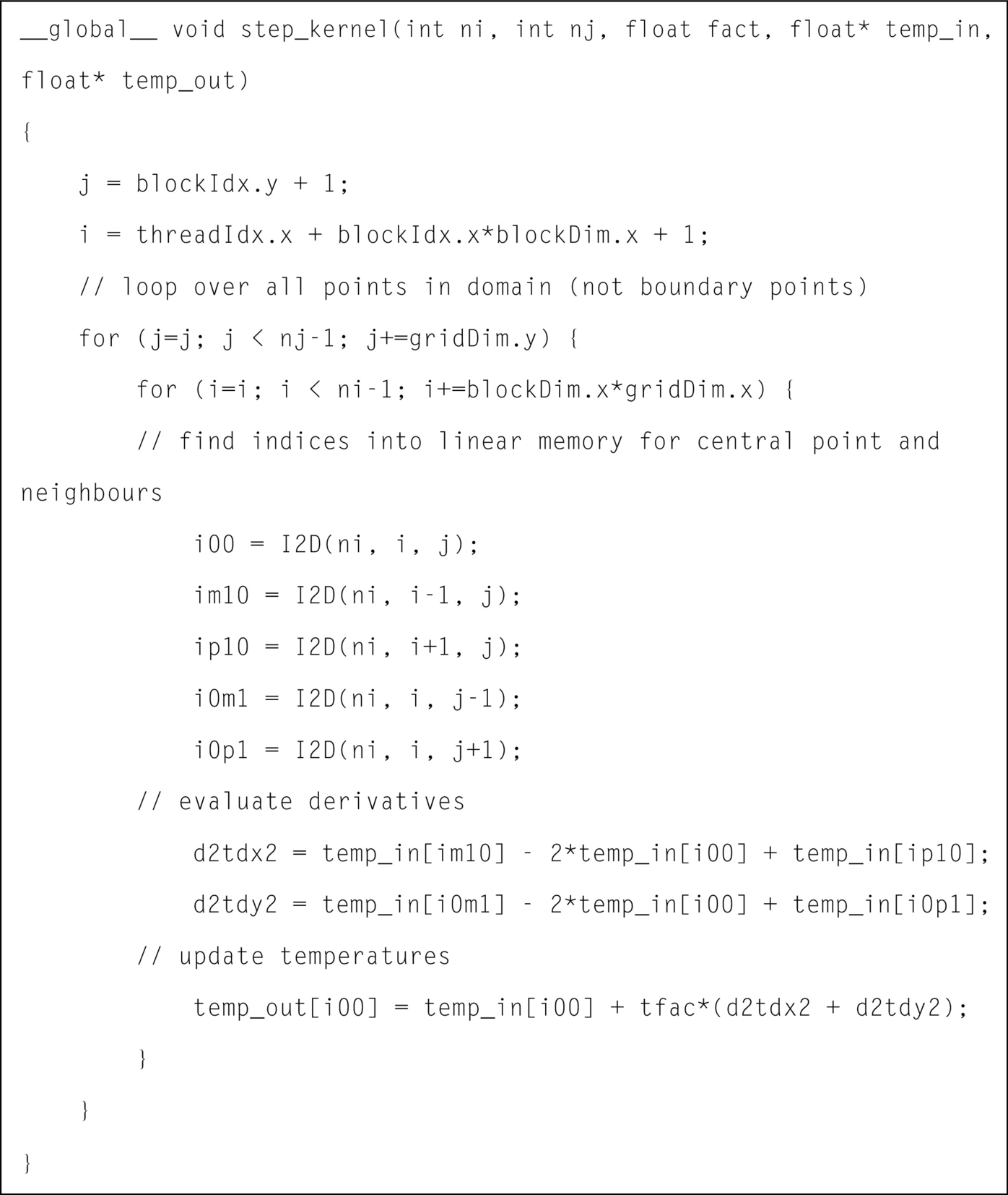
A snippet from our code that implements the stencil-based temperature update is reproduced in Fig. 14. The number of iterations used in our experiments is 20,000, and the grid size is increased gradually from 256 × 256 to 4096 × 4096.
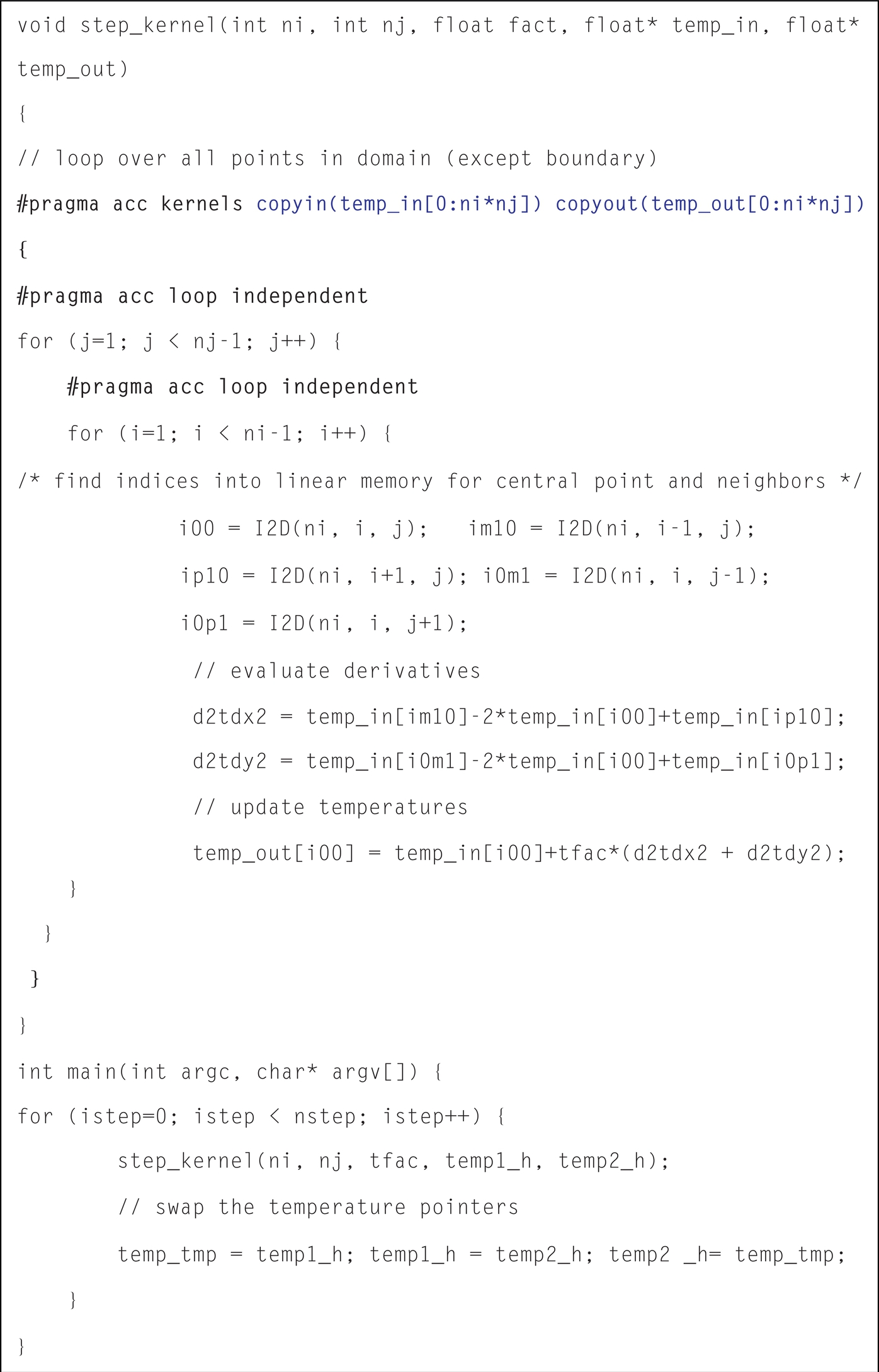
In order to parallelize the application, OpenACC directives are used: “#pragma acc kernels” is inserted at the top of the nested loop inside the temperature updating kernel, and “#pragma acc loop independent” is inserted right before each loop. The “independent” clause is used to tell the compiler that there is no loop-carried dependence in the annotated loop nest. In addition, the copyin and copyout data clauses are added to move the input to GPU and output data from GPU to CPU.
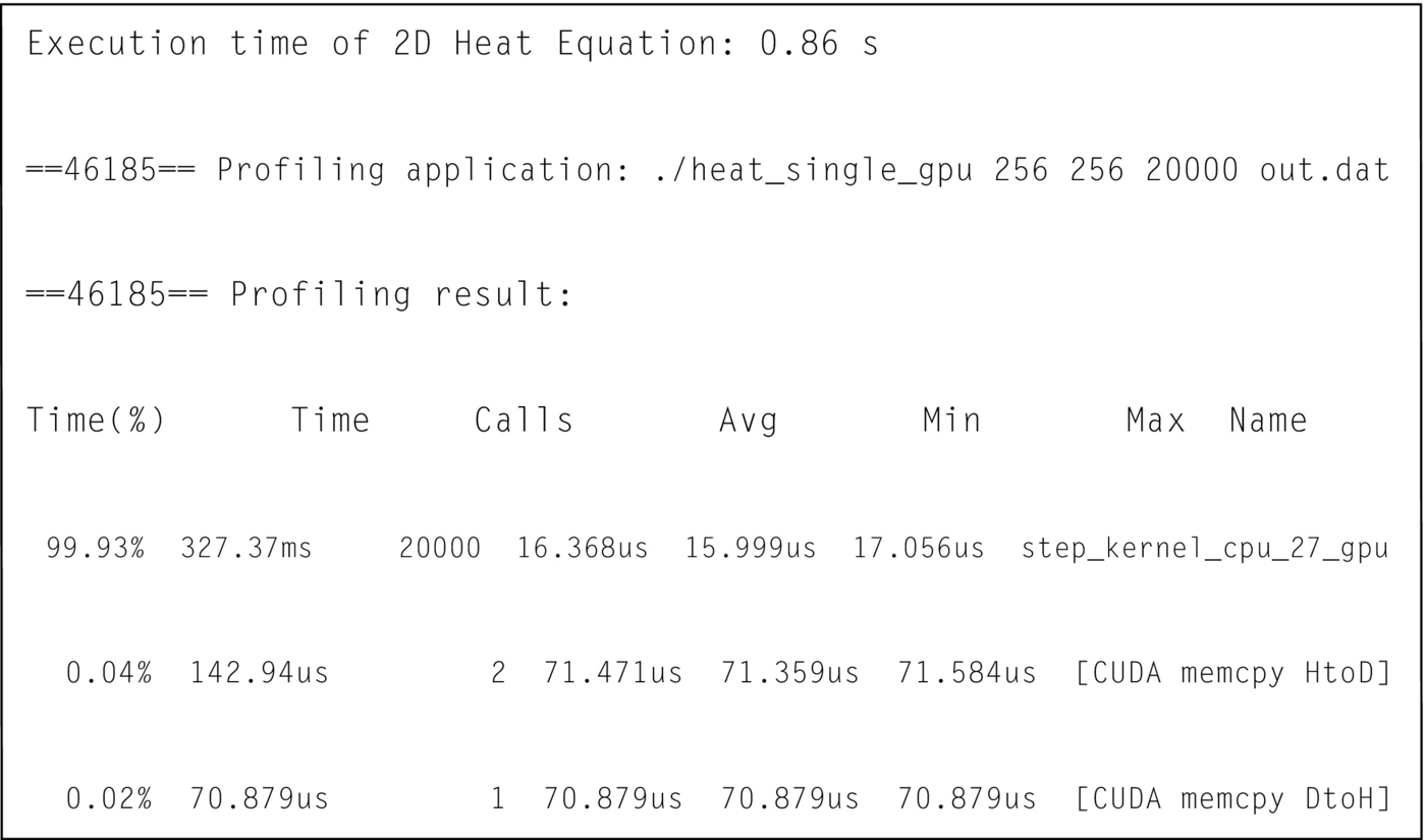
Results of profiling the basic implementation, shown in Fig. 15, indicate that the data is transferred back and forth in every main iteration step.
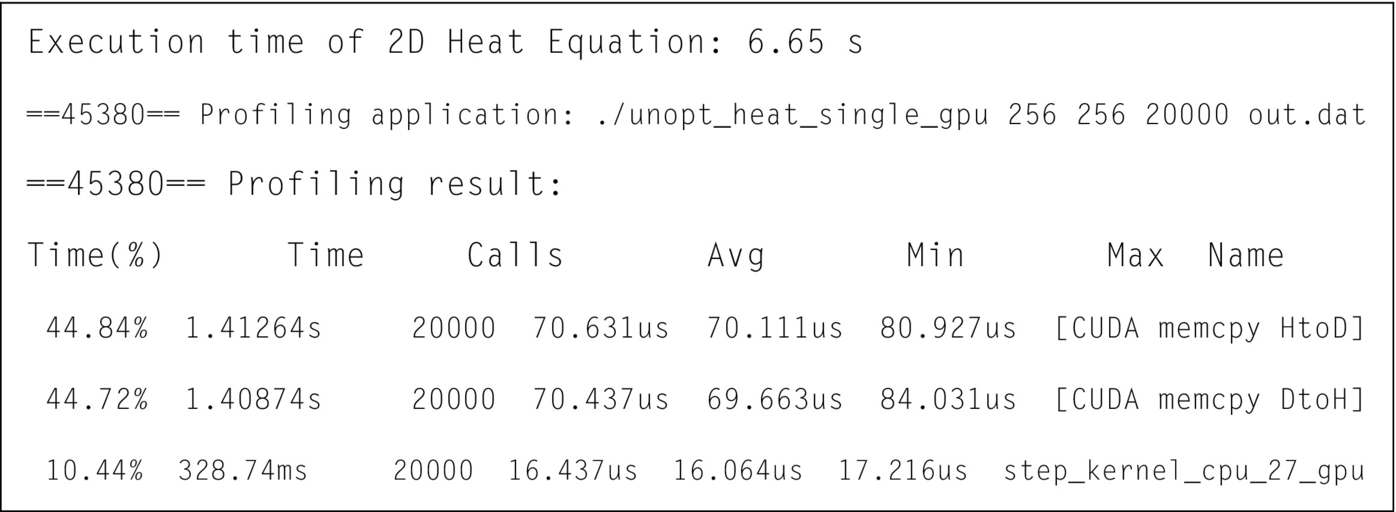
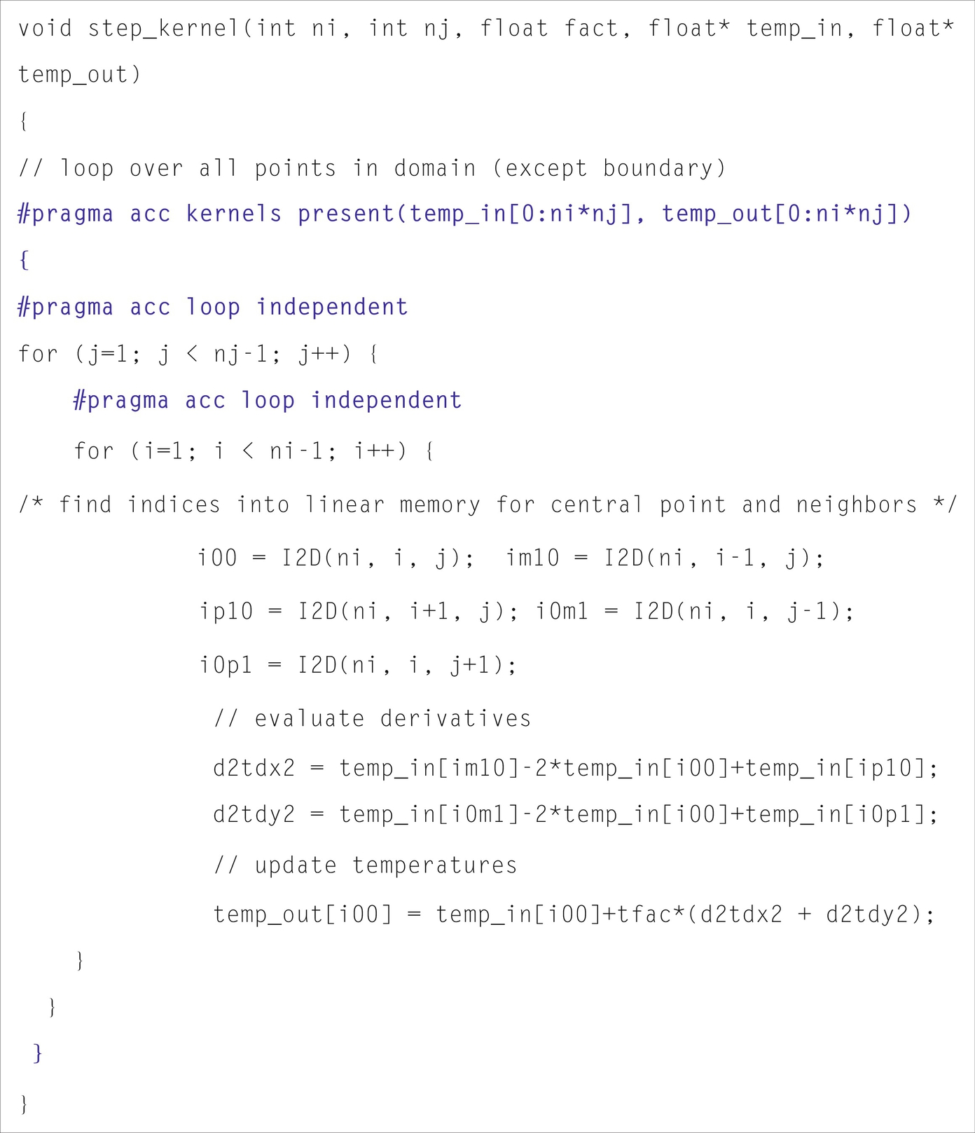
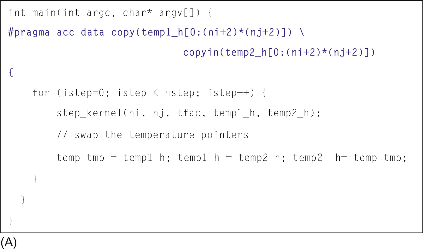
The cost of data transfer is so high that the parallelized code takes longer to execute than the original version on the host. To avoid transferring the data during each step, a data directive is added surrounding the main iterations; this ensures that the data is transferred only before and after the main loops. After all the iterations have completed, the data in temp1 instead of temp2 needs to be transferred from GPU to CPU since the pointers of temp1 and temp2 have been swapped earlier. In the kernel, the copyin and copyout clauses are replaced by the present clause which indicates that the data are already present on the GPU and thus there is no need to do any data movement.
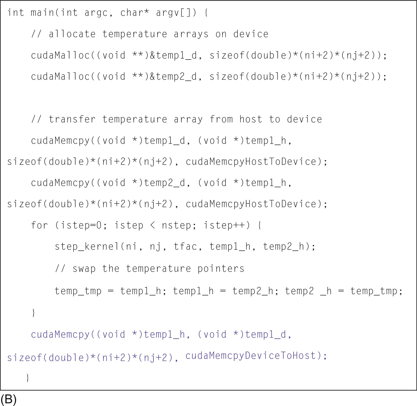
Fig. 16A shows the OpenACC code snippet after applying data optimization and Fig. 17 shows the corresponding profile result. It is clear that the number of times the data is moved has been reduced from 40,000 to only 3. To enable a comparison, Fig. 16B shows a CUDA implementation of the same kernel.
Hybrid OpenMP/OpenACC
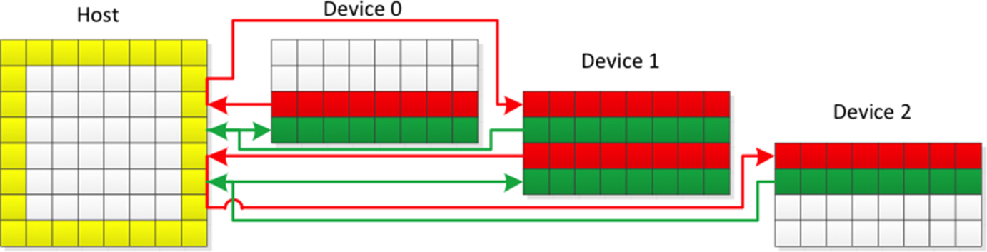
This section discusses the case where the application uses two GPUs. Fig. 18 reproduces the program details including comments. In this implementation, ni and nj are the X and Y dimensions of the grid (not including the boundary), respectively. As can be seen in Fig. 18, the grid is partitioned into two parts along the Y dimension, each of which will run on one GPU. The decomposed parts overlap at the boundaries and the overlapping regions are called halo regions. At the start of the computation, the initial temperature is stored in temp1_h; after updating the temperature, the new temperature is stored in temp2_h. Then the pointer is swapped so that in the next iteration the input of the kernel points to the current new temperature. Since each data point needs temperature values from its neighboring points in the previous iteration for the update, the two GPUs need to exchange halo data at every iteration. With today’s technology, the data cannot be exchanged directly between different GPUs using high-level directives or runtime libraries. The only workaround is to first transfer the data from one device to the host and then from the host to the other device. This is illustrated in Fig. 19 for the 2D heat equation where different OpenACC devices exchange halo data through the CPU.
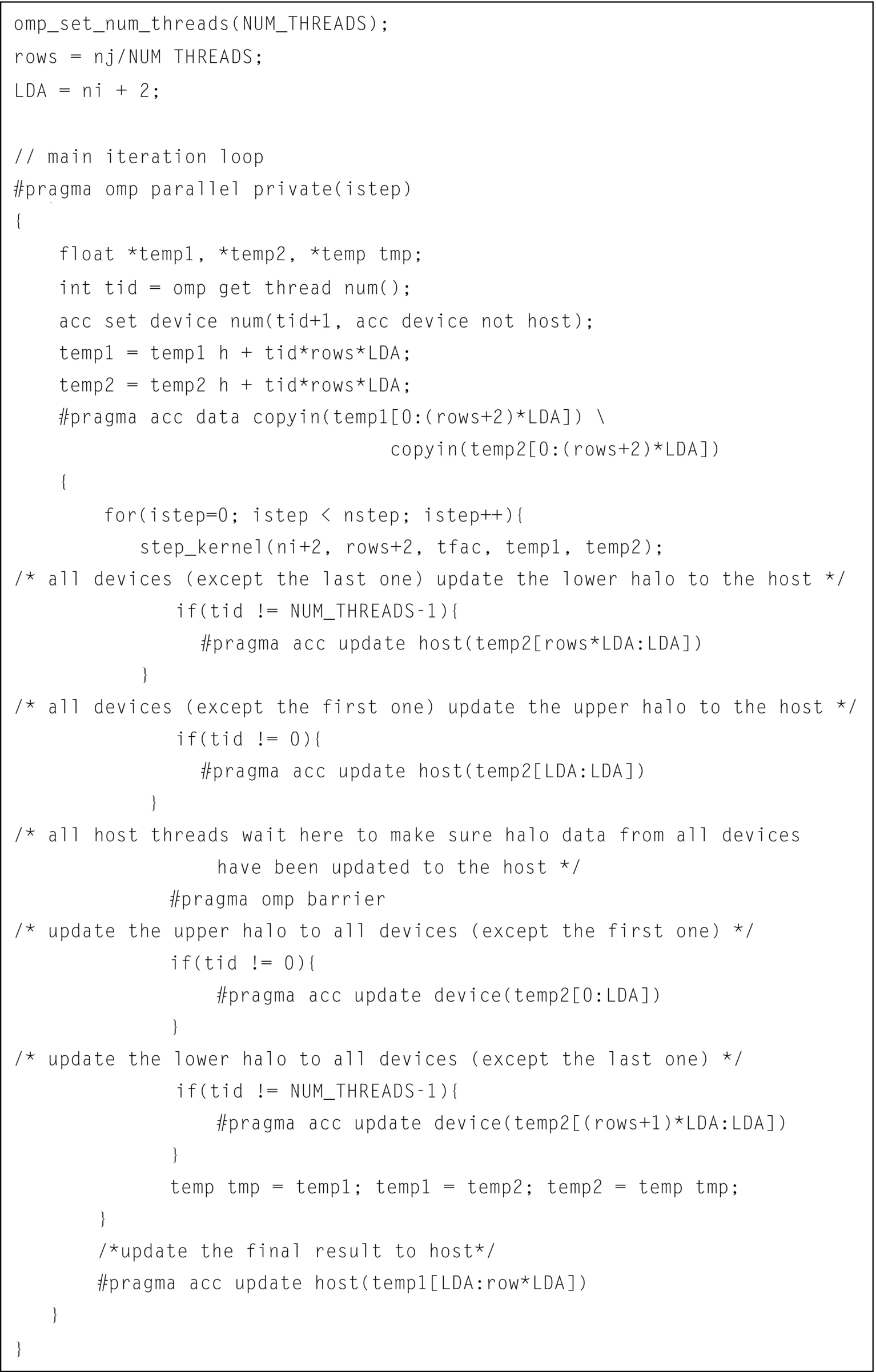
The profiling results in Fig. 20 also confirm that after every iteration, the pair of GPUs exchange data through the CPU. Because different GPUs use different parts of the data in the grid, separate memory for these partial data do not need to be allocated, instead only the private pointer needs to be used to point to the different positions of the shared variable temp1_h and temp2_h. If tid represents the id of a thread, then that thread’s pointer points to the position tid*rows*(ni + 2) of the grid (because it needs to include the halo region) and it needs to transfer (rows + 2)*(ni + 2) data to the device where rows is equal to nj/NUM_THREADS. The kernel that updates the temperature in the multiGPU implementation is exactly the same as the one in the single-GPU version.
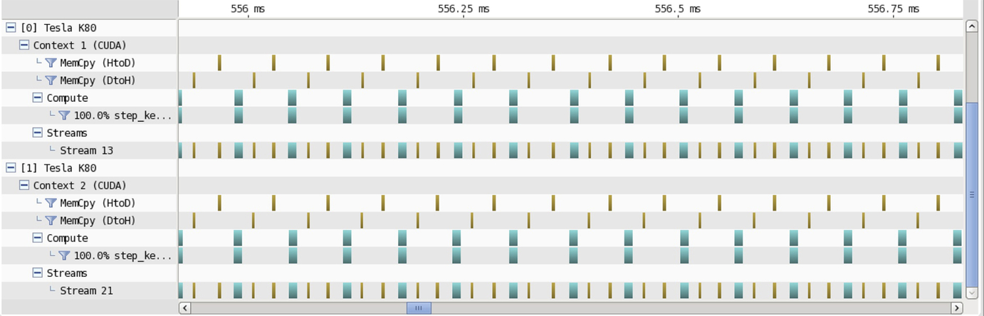
Fig. 21 shows the results of profiling both OpenACC and CUDA multiGPU implementations. Note that their performance is similar. The kernel performance of the OpenACC implementation is slightly better than that of the CUDA implementation, which demonstrates that when translating OpenACC kernels, the OpenACC compiler may apply optimizations that are not available in the CUDA compiler.
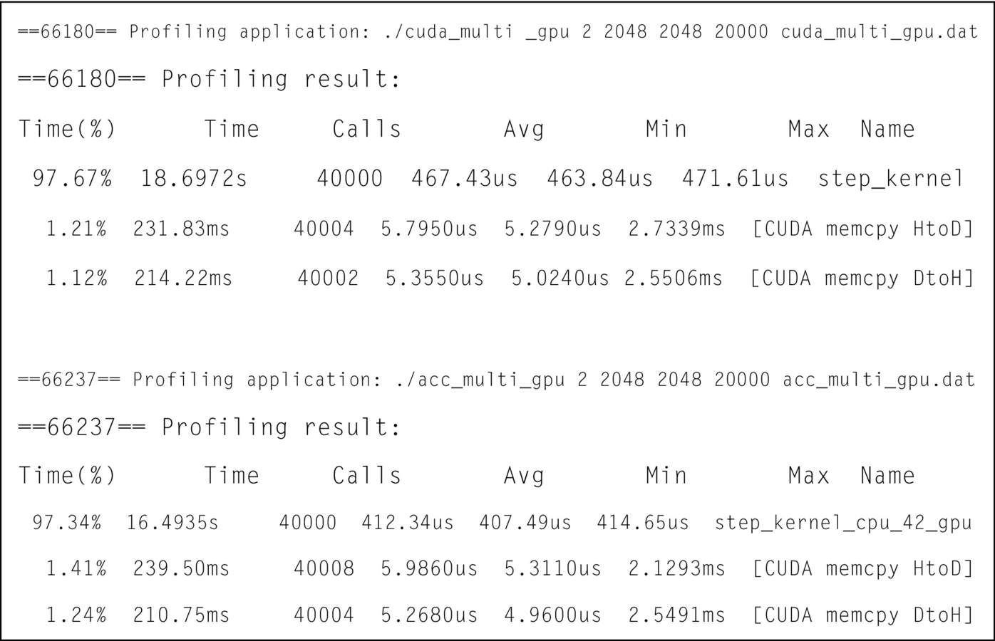
Fig. 22 compares the performance obtained by different implementations. It is obvious that the execution time of the serial version of the code on a single CPU is always the slowest. The OpenACC multicore performance is slightly better than the GPU performance when the problem size is small, but poorer than GPU performance when the problem size is large. While comparing the performance of multiGPU with single GPU, we noticed that there is a trivial performance difference when the problem size is small. However, there is a significant increase in performance using multiple GPUs for larger grid sizes.
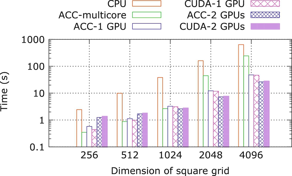
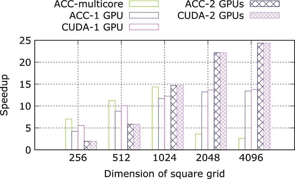
Fig. 23 shows the speedup in multicore and GPU compared to the CPU performance. For a grid size of 4096 × 4096, the speedup obtained using two GPUs is around twice that of the single GPU implementation. This is because as the grid size increases, the computation also increases significantly, while the halo-data exchange remains small. Thus the computation/communication ratio increases; decomposing the computation to utilize multiple GPUs to can be quite advantageous. It is also apparent that the performance of the OpenMP/OpenACC implementation for multiple GPUs is comparable to the CUDA implementation.
Summary
OpenACC, a directive-based programming model, can generate executables for more devices than just GPUs. This means that an application scientist can maintain a single code base whilst porting applications across a range of computing devices. This is critical since legacy codes usually contain several millions of lines of code, and it is impractical to rewrite them every time the device architecture changes. Moreover it is expensive, time-consuming, and effectively impractical to rewrite them in low-level languages such as CUDA or OpenCL.
This chapter showcased some coding challenges and walks the reader through incremental code improvements using OpenACC. The reader will notice that the performance achieved depends primarily on the characteristics of the code, which can be discovered through the use of profiler tools. From our experimental results, we conclude that efficient implementations of high-level directive-based models, plus user-guided optimizations, are capable of producing the same performance as hand-written CUDA code.