Introduction to Pipelining

Synchronous operations require that one operation must wait for another to complete before it can begin. As an example, consider a grocery checkout line: before the customer can pay for their groceries the checkout clerk must finish scanning all of the groceries. Scanning and paying are two distinct operations, but the operation of paying cannot proceed until the operation of scanning the products is complete. This operation is fairly inefficient, since neither the buyer nor payer can do their part of the transaction until the other has completed. To service more customers, it can be tempting to think that the solution is to open more lanes, when in fact a better solution is to optimize what happens within each checkout lane. For instance, a bagger can be busy bagging groceries while the customer is paying, the customer can be preparing the payment while the groceries are being scanned, and the clerk can be scanning one customer’s groceries while the next customer begins loading their groceries onto the conveyor belt. Each of these operations are independent and can, at times, be carried out at the same time, provided they occur in the right order. These are the stages in the grocery checkout pipeline: unload the cart onto the belt, scan the groceries, bag the groceries, and pay. By allowing each person in the process to work asynchronously from each other the checkout line is able to process multiple customers in a more efficient manner than simply opening more checkout lanes.

Another example of a pipeline is an automobile assembly line. While Henry Ford did not invent the automobile, he optimized the way automobiles were produced by recognizing that certain steps in the process could be completed at the same time on different cars, provided the steps always occur in a specific order. For example, one worker welds together the frame, another worker adds wheels to a completed frame, and yet another worker adds the body around the completed frame with wheels. By ensuring that each step in the assembly takes a comparable amount of time, assembly lines are an effective way to keep every worker productive while building an automobile in a predictable amount of time.

We can apply this same concept to an OpenACC program. By default, OpenACC directives operate synchronously between the host CPU and the accelerator, meaning that the host CPU waits (blocks) until the accelerator operation completes before moving forward. By making OpenACC regions asynchronous, however, the CPU can immediately do other things, such as enqueue additional work, perform data transfers, or perform other compute operations on the host. Asynchronous operations enable all parts of the system to be productive: the host CPU, the accelerator, and the PCIe bus, when present, for data transfers. In the case study that follows we use a technique known as pipelining to reduce execution time by overlapping operations that can be done simultaneously to keep the parts of the system busy, much like the assembly line discussed previously.

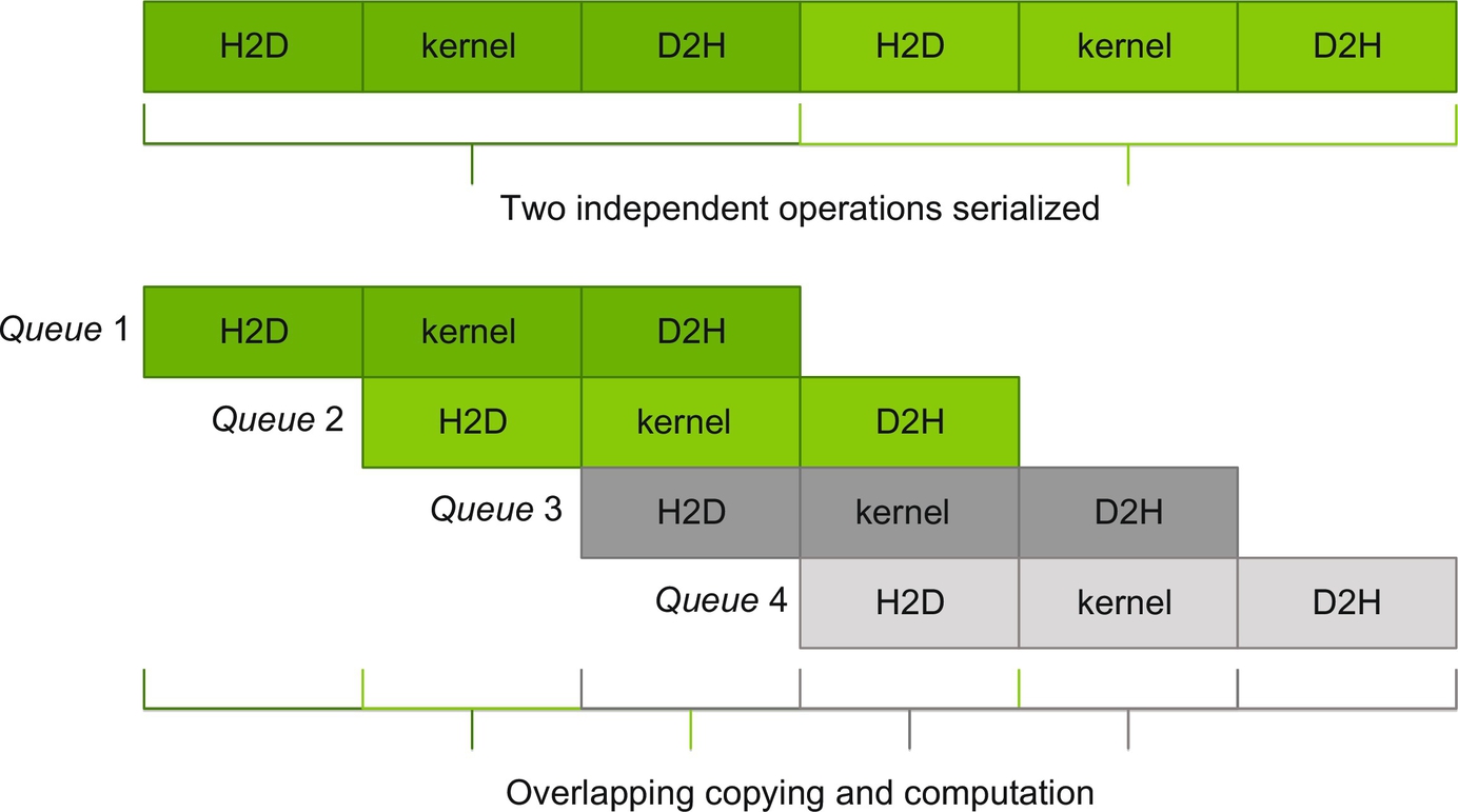
Fig. 1 shows an idealized pipeline that one might build to overlap accelerator computation fully with data transfers, where H2D represents host to device copies and D2H represents device to host copies. The image is idealized because in reality the time taken by each step does not line up as nicely as shown in the picture. Notice that by pipelining the operations four full operations complete in the time two operations would require to execute in serial. Additionally, pipelining limits the full cost (time) of data transfers to only the first and last transfers; all other transfers are essentially free.

Example Code: Mandelbrot Generator

The example code used in this chapter generates a Mandelbrot set like the one shown in Fig. 2. Mandelbrot sets apply a specific formula to each pixel to determine the pixel’s color density. Since each pixel of the image can calculate its color independent of each other pixel, the image generation is ideal for parallel acceleration with OpenACC. The code used in this chapter is licensed under the Apache License, Version 2.0, please read the included license for more details.

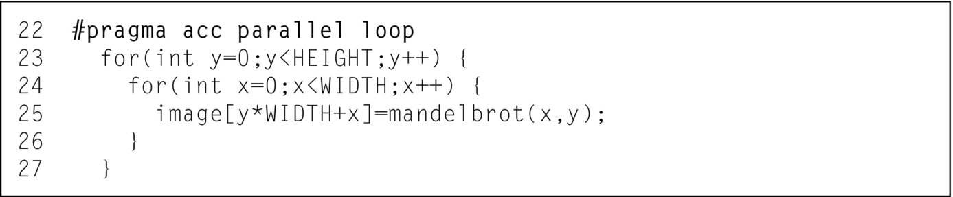
The code is separated into two parts: the loop nest across all pixels in the image and the function that calculates the color of the pixel. The loop nest is in the main function and is accelerated with the OpenACC parallel pragma, although one could have also used the kernels directive. The code is shown in Fig. 3.

Since this requires that the mandelbrot function be called from within an OpenACC region, it is necessary to use the acc routine pragma, as demonstrated in Fig. 4. Notice that this function is called from each and every loop iteration, and it has been declared acc routine seq. This means that the computations within the function are sequential. OpenACC requires that the programmer reserve the parallelism used within routines so that the compiler knows the levels of parallelism that are available for use parallelizing the rest of the code. By declaring the function as sequential, all types of parallelism are available for the loops that call it.

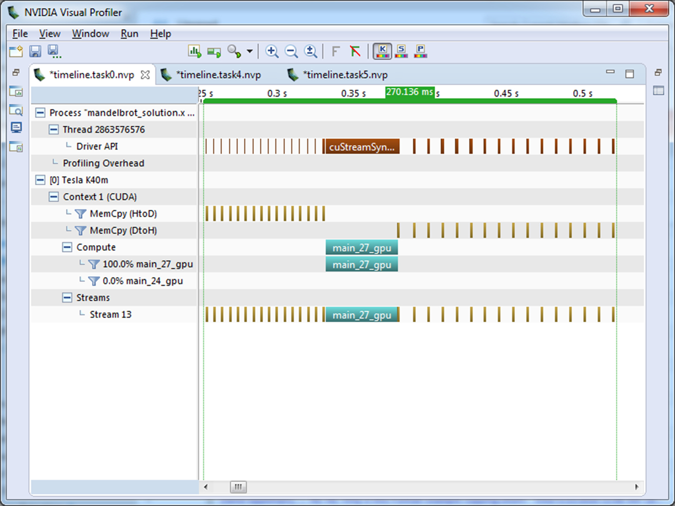
The key to building an effective pipeline is having enough steps, each taking a roughly comparable amount of time, such that each step can be overlapped with other steps. I will be running this test code on a machine with an NVIDIA Tesla K40 GPU. On such a machine there are four operations that can be carried out at the same time: copying data to the GPU over PCIe, copying data from the GPU over PCIe, computing on the GPU, and computing on the CPU. This case study is only able to carry out two operations, however, computing on the GPU and copying data from the GPU memory. This is because the image generation doesn’t require input data, so we can ignore the copy to the GPU. Additionally, in this case study it is difficult to load balance the calculation between the CPU and GPU, so we’ll just ignore the CPU. Fig. 5 shows the Visual Profiler timeline for the current code, notice the PCIe copies before and after the compute kernel.

The initial PCIe copy can be trivially eliminated by adding a copyout data clause, but then we run into a problem with the current code structure. As the code is currently written the copying of the image back to CPU memory can’t occur until the completion of the main_20_gpu kernel. In order the enable the overlapping of computation and PCIe copies it is necessary to use a technique commonly referred to as blocking to break the problem into smaller chunks that can operate independently.

Blocking Computation

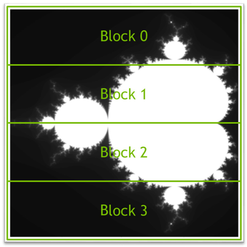
Blocking, or tiling, a computation is a technique of breaking a single large operation into smaller, independent pieces. When blocking is applied correctly, the final result should require the same amount of work and produce the correct results. Fig. 6 shows the same Mandelbrot set image that was generated previously and illustrates the image can be broken into multiple parts, in this case 4, that are generated separately because each pixel is generated independently. For this exercise we only block the image generation along rows, as shown, but the code can also be blocked by columns or by rows and columns. The decision to block by row ensures that the data for each block is contiguous in memory, thus simplifying the transfer of the data to and from the accelerator.

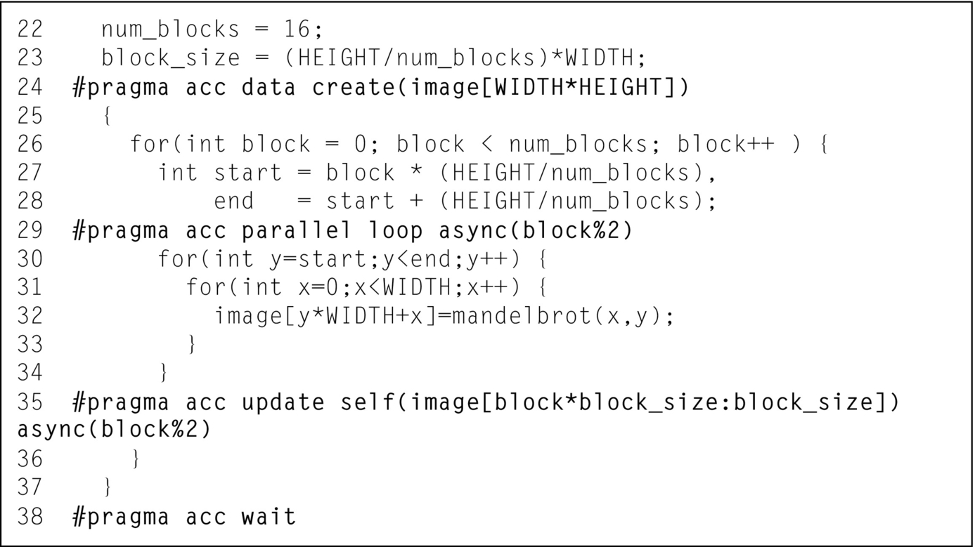
In order to operate in blocks along columns, it is necessary to break the outer, “y” loop into smaller parts by inserting a new outer loop that operates across blocks. The “y” loop now starts at the first row of each chunk and only iterates until the last row of the block. For simplicity we assume that the number of blocks always evenly divides into the height of the image so that the block sizes are always equal. Fig. 7 shows the code for this step, using 16 blocks rather than 4 shown in Fig. 6.

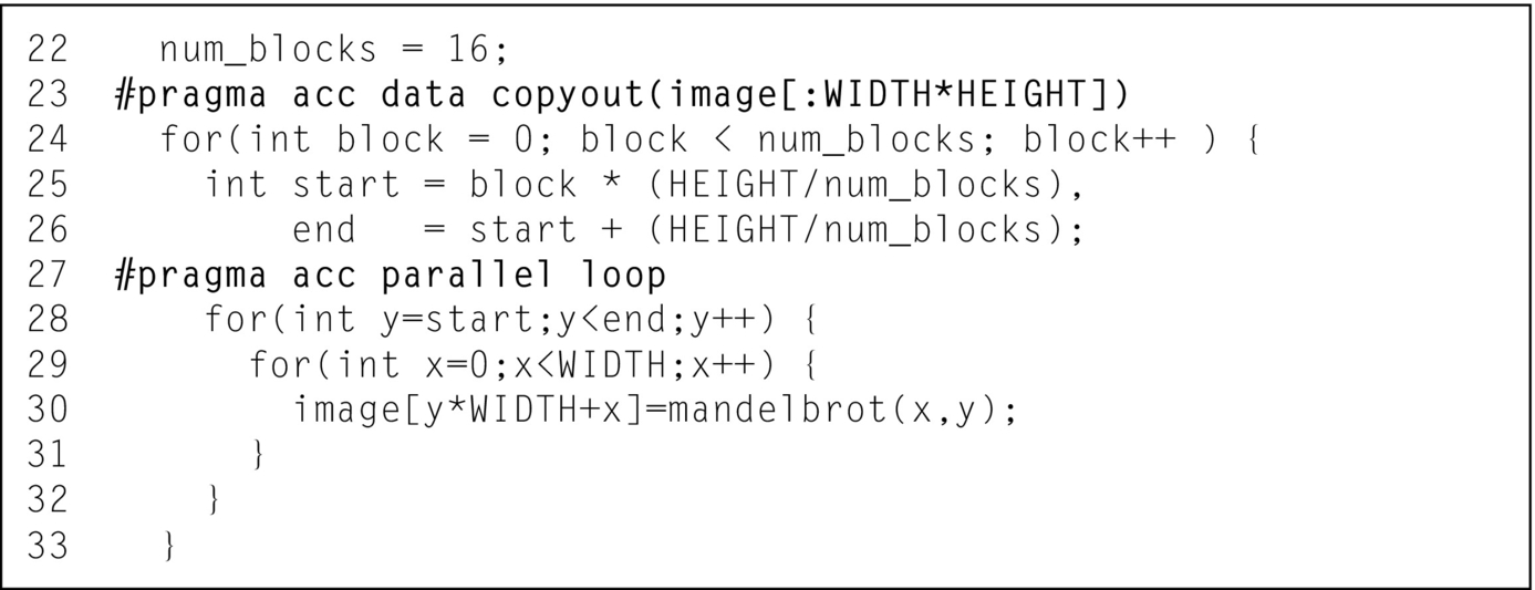
At this point only the computation is blocked, but not the data movement. This is to ensure that if mistakes are made in figuring out the starting and ending values for the “y” loop then the mistakes are found and corrected early. Line 22 specifies the number of blocks to use in the “y” dimension. Line 23 adds a data region to ensure that the image array is only copied back to the host after all parallel loops finish executing on the accelerator. Lines 25 and 26 calculate the starting and ending value for the “y” loop respectively. Finally, line 28 is the modified loop, which iterates only over the rows in each block. Note that building and running the code at this step should still produce the correct image and should run in roughly the same amount of time as the previous step.

Blocking Data Copies

The next step in building the Mandelbrot pipeline is to block the data transfers in the same way as the computation. First add an update directive after the “y” loop, but before the end of the blocking loop. This directive copies only the part of the image array operated on by the current block. The starting value and count (or starting and ending value in Fortran) can be tricky, since they need to account for the width of each row, not just the number of rows. Line 34 in Fig. 8 shows the correct update directive. Lastly the data clause on line 24 must be changed from a copyout to a create, since the data transfers are now handled by the update directive. Fig. 8 shows the complete code for this step.

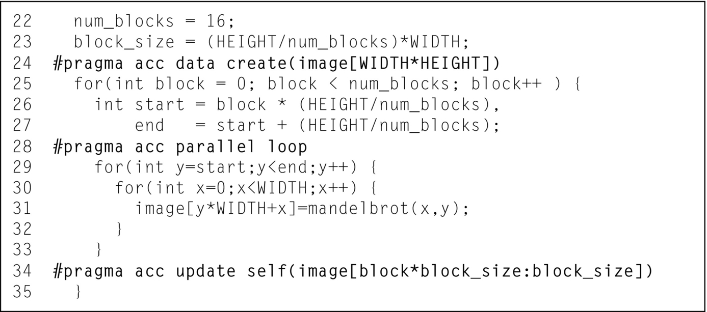
Once again, it is important to rebuild and rerun the code to ensure that the code still produces correct results. The runtime of the code at this step should be roughly comparable to the original runtime, since we have not yet introduced overlapping.

Asynchronous Execution

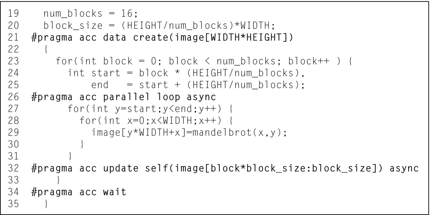
Now that both the computation and data transfers have been blocked they can be made asynchronous, freeing the host CPU to issue each block to the accelerator without waiting for the previous block to complete. This is done by using the async clause and wait directive. The async clause can be added to nearly any OpenACC directive to make it operate asynchronously with the CPU. When a directive includes the async clause the operation of that directive is placed in a work queue and execution immediately returns to the host CPU. Since all of the accelerator directives are now operating asynchronously with the host CPU, the CPU eventually reaches a point at which it needs the results. It is necessary to use the OpenACC wait directive to suspend host execution until the previously issued asynchronous operations complete. In the example code the right place to wait is between the end of the blocking loop and the end of the data region, since we need to ensure that all of the blocks are copied back to the host before the device arrays are destroyed at the end of the data region. Once all asynchronous operations are complete, the host CPU execution can use the results. Fig. 9 shows the resulting code.

The final step in building the pipeline is to exploit the fact that each block is independent of each other block by putting blocks into different asynchronous queues. The async clause accepts a number representing the number of the queue in which to add the work. In theory each block could be given its own queue, but the creation of work queues can be an expensive operation on some architectures. Instead we use just two queues: one queue for computing and one queue for copying data back from the accelerator. The parallel loop and the update for each block must occur in order, so those should occur in the same queue, but different blocks are independent, so they may be placed in different queues. A convenient way to represent the queue number is to use the block number modulo the number of work queues. Fig. 10 shows the resulting code. The wait directive also accepts a queue number, but in this case we do not specify a queue number so the directive waits on all work queues to complete.

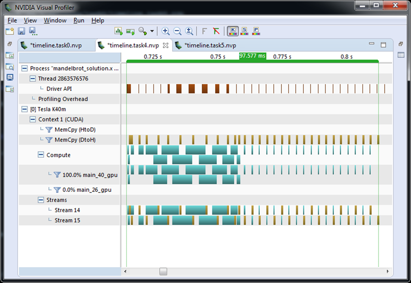
At this point the execution time should be at least slightly improved from the original execution time, since the data copies and computation are now overlapped. The execution can be further improved by varying the number of blocks, which in turn varies the size of each block. Since it is necessary to find a balance between the added overhead of a large number of blocks and the benefit of overlapping small, evenly sized blocks, one should experiment to find the optimal number of blocks for a given system. The best number of blocks differs from system to system due to differences in the accelerator, host CPU, and data transfer speeds. Fig. 11 shows the Visual Profiler timeline with 16 blocks on an NVIDIA Tesla K40 GPU.

Pipelining Across Multiple Devices

Since the image generation is now divided into independent blocks, it is not only possible to pipeline the blocks on a single accelerator, but the blocks could actually be executed across multiple devices. OpenACC provides an API for selecting which device the runtime should use based on a device type and number. Up to this point the example has used the default device, which is selected automatically by the runtime. It is possible to change which device the runtime uses by calling the acc_set_device_num function.

Multiple devices can be managed in a variety of different ways, including using the same CPU thread to manage all devices, using different processes per GPU, or using different threads. In this example the technique that requires the least code changes is to use OpenMP threads on the CPU to divide the blocks and assign each OpenMP thread to one of the available devices. Since the image array is small enough to fit in the memory of a single GPU, we simply replicate the entire image array on each device. When the data is too large to fit in a single accelerator’s memory additional changes are required to only allocate enough space per accelerator to hold its part of the operation.

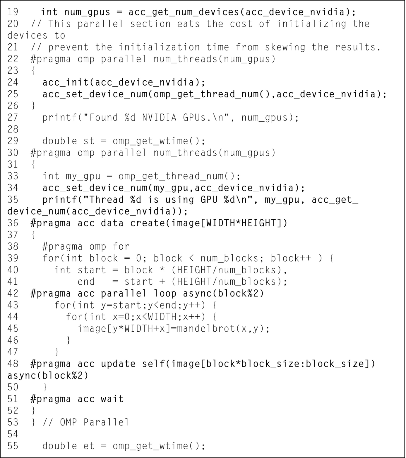
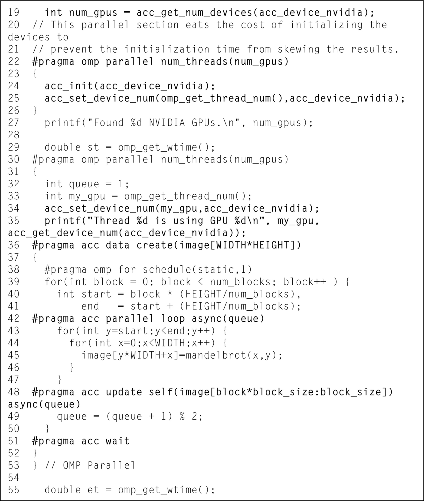
The PGI compiler used in this example allows using OpenACC and OpenMP in the same program, as long as they are not used on the same loop. In this example, OpenMP is used strictly on the blocking loop to workshare blocks to OpenMP threads and OpenACC is used for data management and for the “x” and “y” loops within each block. OpenMP must be enabled at compile-time using the –mp command line option. Fig. 12 shows how to use an OpenMP parallel construct to generate one thread per available device (line 22), using the acc_get_num_devices function (line 19) to query how many devices are available, and assign each thread a unique device (line 35). Each device still uses two asynchronous queues to enable overlapping of data transfers and computation.

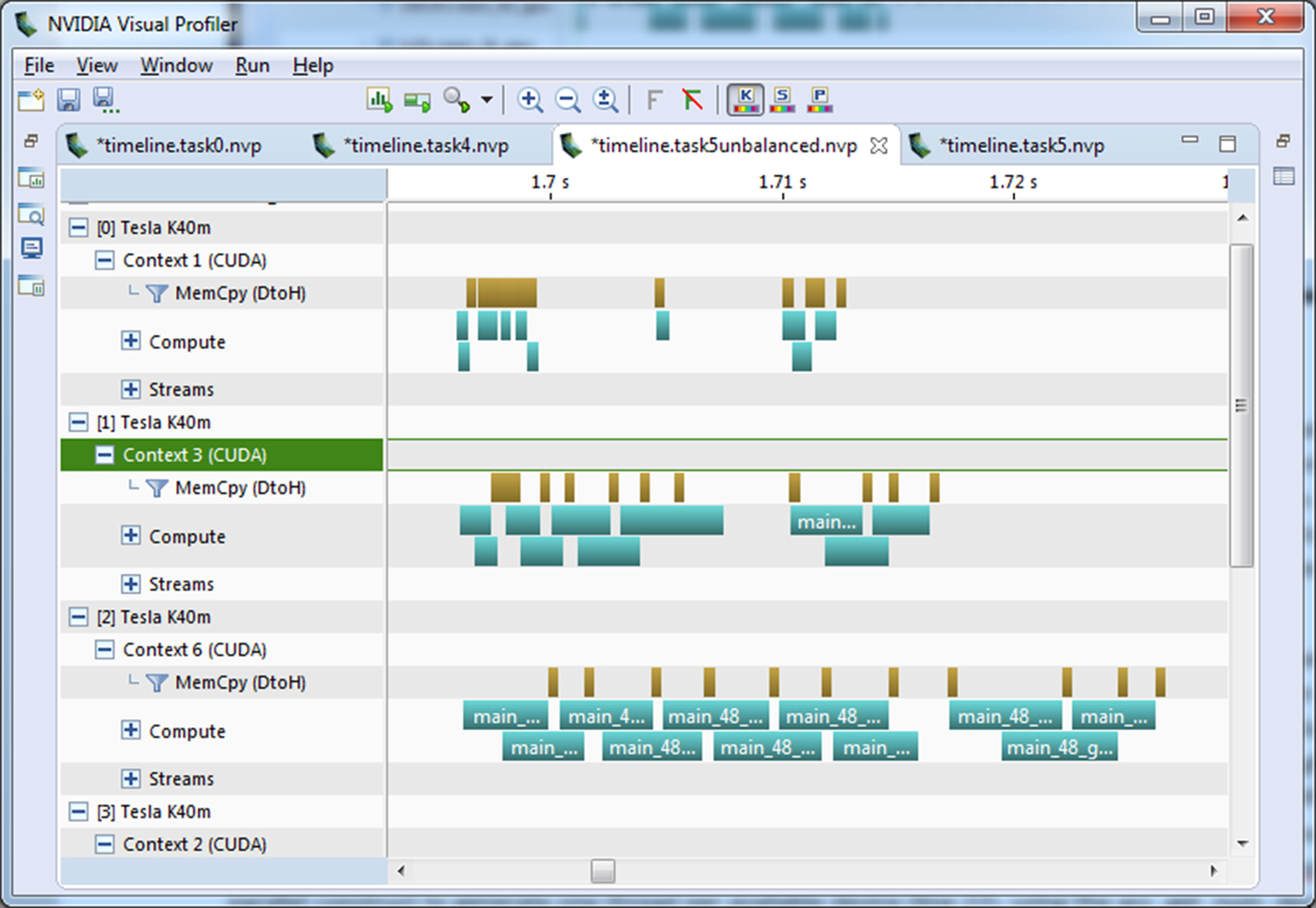
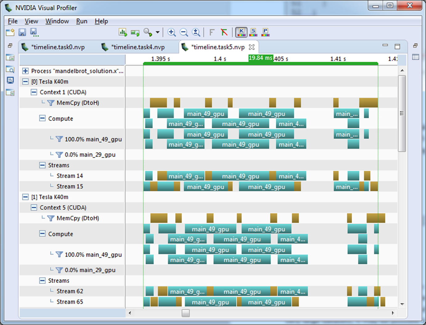
Inspecting the GPU timeline using Visual Profiler (Fig. 13) reveals something peculiar. When run on 6 devices, devices 0 and 5 execute very quickly, while devices 1, 2, 3, and 4 execute relatively slowly. This phenomenon is due to an inherent load imbalance in the Mandelbrot generation. Looking at Fig. 2 notice that the middle part of the image is mostly white, while the outside of the image is mostly black. The white area in the Mandelbrot image indicates more iterations of the loop inside the mandelbrot function, meaning that the inner area takes longer to generate than the outer. In order to see the benefit of the multiple devices it is necessary to better balance the work between the devices. Most applications do not have such a load imbalance, so this next optimization is specific to this example code.

In order to load balance the four accelerators better, we change the way the blocks are assigned to each device. Since we are using OpenMP to assign the iterations of the block loops to different threads, and thus different devices, the simplest way to reassign the blocks is to change the schedule of the OpenMP loop. Using a static schedule with a chunksize of 1 assigns the loop iterations in a round robin manner to the devices rather than assigning contiguous chunks. One side effect of this change is that even and odd numbered threads only receive even and odd numbered blocks respectively. This change makes our logic to assign asynchronous queues insufficient to observe overlapping. Fortunately, this is easily fixed by introducing an additional variable to maintain the queue number within each thread. Fig. 14 shows the resulting code. Fig. 15 shows the final Visual Profiler timeline.

Conclusions

Pipelining is a powerful technique to take advantage of OpenACC’s asynchronous capabilities to overlap computation and data transfer to speed up a code. On the reference system adding pipelining to the code results in a 2.9× speed-up and extending the pipeline across six devices increases this speed-up to 7.8× over the original. Pipelining is just one way to write asynchronous code, however. For stencil types of codes, such as finite difference and spectral element methods, asynchronous behavior may be used to overlap the exchange of boundary conditions with calculations on interior elements. When working on very large datasets, it may be possible to use asynchronous coding to divide the work between the host CPU and accelerator or to perform out-of-core calculations to stream the data through the accelerator in smaller chunks. Writing asynchronous code requires a lot of forethought and careful coding, but the end result is often better utilization of all available system resources and improved time to solution.