
Chapter Six
Geometry of Positive Matrices
The set of n × n positive matrices is a differentiable manifold with a natural Riemannian structure. The geometry of this manifold is intimately connected with some matrix inequalities. In this chapter we explore this connection. Among other things, this leads to a deeper understanding of the geometric mean of positive matrices.
6.1 THE RIEMANNIAN METRIC
The space ![]() is a Hilbert space with the inner product
is a Hilbert space with the inner product ![]() = tr A∗B and the associated
norm ||A||2 = (tr A∗A)1/2. The set of Hermitian matrices constitutes a real vector
space
= tr A∗B and the associated
norm ||A||2 = (tr A∗A)1/2. The set of Hermitian matrices constitutes a real vector
space ![]() in
in ![]() . The subset
. The subset ![]() consisting of strictly positive matrices is an open subset
in
consisting of strictly positive matrices is an open subset
in ![]() . Hence it is a differentiable manifold. The tangent space to
. Hence it is a differentiable manifold. The tangent space to ![]() at any of its points
A is the space
at any of its points
A is the space ![]() , identified for simplicity, with
, identified for simplicity, with ![]() . The inner product on
. The inner product on ![]() leads to
a Riemannian metric on the manifold
leads to
a Riemannian metric on the manifold ![]() . At the point A this metric is given by the
differential
. At the point A this metric is given by the
differential
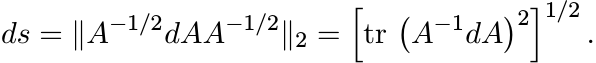 (6.1)
(6.1)
This is a mnemonic for computing the length of a (piecewise) differentiable path
in ![]() . If
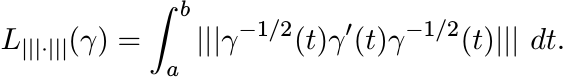
. If ![]() is such a path, we define its length as
is such a path, we define its length as
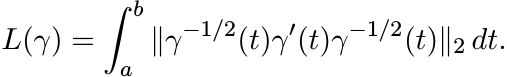 (6.2)
(6.2)
For each X ∈ GL(n) the congruence transformation ΓX(A) = X∗AX is a bijection of ![]() onto itself. The composition ΓX ◦ γ is another differentiable path in
onto itself. The composition ΓX ◦ γ is another differentiable path in ![]() .
.
6.1.1 Lemma
For each X ∈ GL(n) and for each differentiable path γ
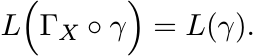 (6.3)
(6.3)Proof. Using the definition of the norm || · ||2 and the fact that tr XY = tr Y X for all X and Y we have for each t
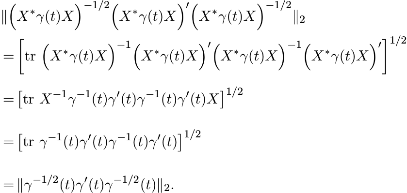
Intergrating over t we get (6.3). ■
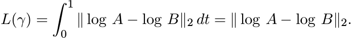
For any two points A and B in ![]() let
let
This gives a metric on ![]() . The triangle inequality
. The triangle inequality
is a consequence of the fact that a path γ1 from A to C can be adjoined to a path γ2 from C to B to obtain a path from A to B. The length of this latter path is L(γ1) + L(γ2).
According to Lemma 6.1.1 each ΓX is an isometry for the length L. Hence it is also an isometry for the metric δ2; i.e.,
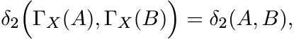 (6.5)
(6.5)
for all A, B in ![]() and X in GL(n).
and X in GL(n).
This observation helps us to prove several properties of δ2. We will see that the
infimum in (6.4) is attained at a unique path joining A and B. This path is called
the geodesic from A to B. We will soon obtain an explicit formula for this geodesic
and for its length. The following inequality called the infinitesimal exponential
metric increasing property (IEMI) plays an important role. Following the notation
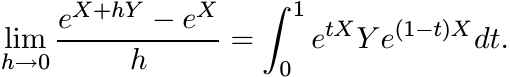
introduced in Exercise 2.7.15 we write DeH for the derivative of the exponential
map at a point H of ![]() . This is a linear map on
. This is a linear map on ![]() whose action is given as
whose action is given as

6.1.2 Proposition (IEMI)
For all H and K in Hn we have
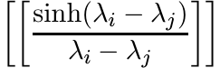
Proof. Choose an orthonormal basis in which H = diag (λ1, . . . , λn). By the formula (2.40)
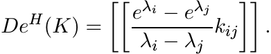
Therefore, the i, j entry of the matrix e−H/2 D eH(K) e−H/2 is
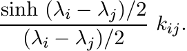
Since (sinh x)/x ≥ 1 for all real x, the inequality (6.6) follows. ■
6.1.3 Corollary
Let H(t), a ≤ t ≤ b be any path in Hn and let γ(t) = eH(t). Then
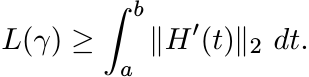 (6.7)
(6.7)
Proof. By the chain rule ![]() . So the inequality (6.7) follows from the definition of
L(γ) given by (6.2) and the IEMI (6.6). ■
. So the inequality (6.7) follows from the definition of
L(γ) given by (6.2) and the IEMI (6.6). ■
If γ(t) is any path joining A and B in ![]() , then H(t) = log γ(t) is a path joining log
A and log B in
, then H(t) = log γ(t) is a path joining log
A and log B in ![]() . The right-hand side of (6.7) is the length of this path in the Euclidean
space
. The right-hand side of (6.7) is the length of this path in the Euclidean
space ![]() . This is bounded below by the length of the straight line segment joining
log A and log B. Thus L(γ) ≥ || log A − log B||2, and we have the following important
corollary called the exponential metric increasing property (EMI).
. This is bounded below by the length of the straight line segment joining
log A and log B. Thus L(γ) ≥ || log A − log B||2, and we have the following important
corollary called the exponential metric increasing property (EMI).
6.1.4 Theorem (EMI)
For each pair of points A, B in ![]() we have
we have
In other words for any two matrices H and K in ![]()
So the map
increases distances, or is metric increasing.
Our next proposition says that when A and B commute there is equality in (6.8). Further
the exponential map carries the line segment joining log A and log B in ![]() to the geodesic
joining A and B in
to the geodesic
joining A and B in ![]() . A bit of notation will be helpful here. We write [H, K] for
the line segment
. A bit of notation will be helpful here. We write [H, K] for
the line segment
joining two points H and K in ![]() . If A and B are two points in
. If A and B are two points in ![]() we write [A, B] for
the geodesic from A to B. The existence of such a path is yet to be established.
This is done first in the special case of commuting matrices.
we write [A, B] for
the geodesic from A to B. The existence of such a path is yet to be established.
This is done first in the special case of commuting matrices.
6.1.5 Proposition
Let A and B be commuting matrices in ![]() . Then the exponential function maps the line
segment [log A, log B] in
. Then the exponential function maps the line
segment [log A, log B] in ![]() to the geodesic [A, B] in
to the geodesic [A, B] in ![]() . In this case
. In this case
Proof. We have to verify that the path

is the unique path of shortest length joining A and B in the space ![]() . Since A and
B commute, γ(t) = A1−tBt and γ′(t) = (log B − log A) γ(t). The formula (6.2) gives
in this case
. Since A and
B commute, γ(t) = A1−tBt and γ′(t) = (log B − log A) γ(t). The formula (6.2) gives
in this case
The EMI (6.7) says that no path can be shorter than this. So the path γ under consideration is one of shortest possible length.
Suppose ![]() is another path that joins A and B and has the same length as that of γ.
Then
is another path that joins A and B and has the same length as that of γ.
Then ![]() is a path that joins log A and log B in Hn, and by Corollary 6.1.3 this path
has length || log A − log B||2. But in a Euclidean space the straight line segment
is the unique shortest path between two points. So
is a path that joins log A and log B in Hn, and by Corollary 6.1.3 this path
has length || log A − log B||2. But in a Euclidean space the straight line segment
is the unique shortest path between two points. So ![]() is a reparametrization of the
line segment [log A, log B] . ■
is a reparametrization of the
line segment [log A, log B] . ■
Applying the reasoning of this proof to any subinterval [0, a] of [0, 1] we see that the parametrization
of the line segment [log A, log B] is the one that is mapped isometrically onto [A, B] along the whole interval. In other words the natural parametrisation of the geodesic [A, B] when A and B commute is given by
in the sense that δ2 ![]() A, γ(t)
A, γ(t) ![]() = tδ2(A, B) for each t. The general case is obtained
from this with the help of the isometries ΓX.
= tδ2(A, B) for each t. The general case is obtained
from this with the help of the isometries ΓX.
6.1.6 Theorem
Let A and B be any two elements of ![]() . Then there exists a unique geodesic [A, B] joining
A and B. This geodesic has a parametrization
. Then there exists a unique geodesic [A, B] joining
A and B. This geodesic has a parametrization
 (6.11)
which is natural in the sense that
for each t. Further, we have
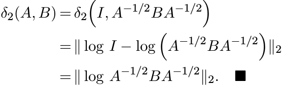
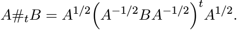
Proof. The matrices I and A−1/2BA−1/2 commute. So the geodesic ![]() is naturally parametrized
as
is naturally parametrized
as

Applying the isometry ΓA1/2 we obtain the path

joining the points ΓA1/2(I) = A and ΓA1/2 ![]() A−1/2BA−1/2
A−1/2BA−1/2![]() = B. Since ΓA1/2 is an isometry
this path is the geodesic [A, B]. The equality (6.12) follows from the similar property
for γ0(t) noted earlier. Using Proposition 6.1.5 again we see that
= B. Since ΓA1/2 is an isometry
this path is the geodesic [A, B]. The equality (6.12) follows from the similar property
for γ0(t) noted earlier. Using Proposition 6.1.5 again we see that
Formula (6.13) gives an explicit representation for the metric δ2 that we defined
via (6.4). This is the Riemannian metric on the manifold ![]() . From the definition of
the norm || · ||2 we see that
. From the definition of
the norm || · ||2 we see that
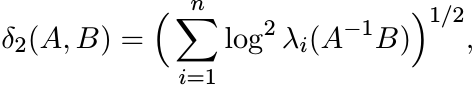 (6.14)
where λi are the eigenvalues of the matrix A−1B.
6.1.7 The geometric mean again
The expression (4.10) defining the geometric mean A#B now appears in a new light.
It is the midpoint of the geodesic γ joining A and B in the space ![]() . This is evident
from (6.11) and (6.12). The symmetry of A#B in the two arguments A and B that we
deduced by indirect arguments in Section 4.1 is now revealed clearly: the midpoint
of the geodesic [A, B] is the same as the midpoint of [B, A].
. This is evident
from (6.11) and (6.12). The symmetry of A#B in the two arguments A and B that we
deduced by indirect arguments in Section 4.1 is now revealed clearly: the midpoint
of the geodesic [A, B] is the same as the midpoint of [B, A].
The next proposition supplements the information given by the EMI.
6.1.8 Proposition
If for some ![]() , the identity matrix I lies on the geodesic [A, B], then A and B commute,
[A, B] is the isometric image under the exponential map of a line segment through
O in
, the identity matrix I lies on the geodesic [A, B], then A and B commute,
[A, B] is the isometric image under the exponential map of a line segment through
O in ![]() , and
, and
 (6.15)
where ξ = δ2(A, I)/δ2(A, B).
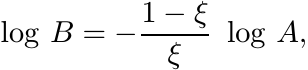
Proof. From Theorem 6.1.6 we know that
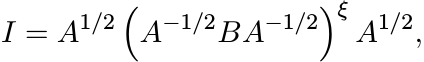
where ξ = δ2 (A, I) /δ2(A, B). Thus
So A and B commute and (6.15) holds. Now Proposition 6.1.5 tells us that the exponential map sends the line segment [log A, log B] isometrically onto the geodesic [A, B]. The line segment contains the point O = log I. ■
While the EMI says that the exponential map (6.10) is metric nondecreasing in general,
Proposition 6.1.8 says that this map is isometric on line segments through O. This
essentially captures the fact that ![]() is a Riemannian manifold of nonpositive curvature.
See the discussion in Section 6.5.
is a Riemannian manifold of nonpositive curvature.
See the discussion in Section 6.5.
Another essential feature of this geometry is the semiparallelogram law for the metric
δ2. To understand this recall the parallelogram law in a Hilbert space ![]() . Let a and
b be any two points in
. Let a and
b be any two points in ![]() and let m = (a + b)/2 be their midpoint. Given any other
point c consider the parallelogram one of whose diagonals is [a, b] and the other
[c, d]. The two diagonals intersect at m
and let m = (a + b)/2 be their midpoint. Given any other
point c consider the parallelogram one of whose diagonals is [a, b] and the other
[c, d]. The two diagonals intersect at m
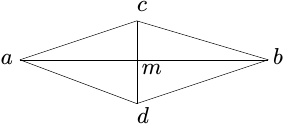
and the parallelogram law is the equality

Upon rearrangement this can be written as
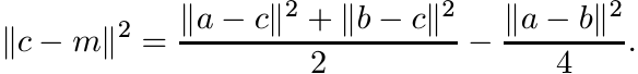
In the semiparallelogram law this last equality is replaced by an inequality.
6.1.9 Theorem (The Semiparallelogram Law)
Let A and B any two points of ![]() and let M = A#B be the midpoint of the geodesic [A,
B]. Then for any C in
and let M = A#B be the midpoint of the geodesic [A,
B]. Then for any C in ![]() we have
we have
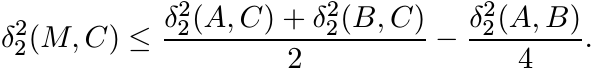 (6.16)
Proof. Applying the isometry ΓM−1/2 to all matrices involved, we may assume that M = I. Now I is the midpoint of [A, B] and so by Proposition 6.1.8 we have log B = − log A and
The same proposition applied to [M, C] = [I, C] shows that
The parallelogram law in the Hilbert space ![]() tells us
tells us
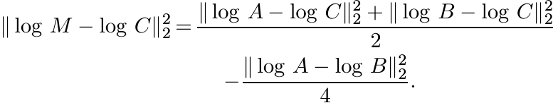
The left-hand side of this equation is equal to ![]() and the subtracted term on the
right-hand side is equal to
and the subtracted term on the
right-hand side is equal to ![]() . So the EMI (6.8) leads to the inequality (6.16). ■
. So the EMI (6.8) leads to the inequality (6.16). ■
In a Euclidean space the distance between the midpoints of two sides of a triangle is equal to half the length of the third side. In a space whose metric satisfies the semiparallelogram law this is replaced by an inequality.
6.1.10 Proposition
Let A, B, and C be any three points in ![]() . Then
. Then
 (6.17)
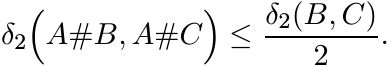
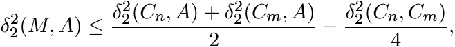
Proof. Consider the triangle with vertices A, B and C (and sides the geodesic segments joining the vertices). Let M1 = A#B. This is the midpoint of the side [A, B] opposite the vertex C of the triangle {A, B, C}. Hence, by (6.16)
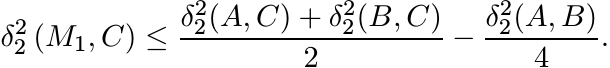
Let M2 = A#C. In the triangle {A, M1, C} the point M2 is the midpoint of the side [A, C] opposite the vertex M1. Again (6.16) tells us
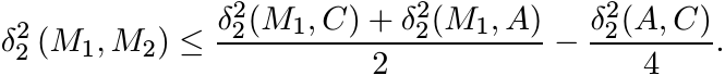
Substituting the first inequality into the second we obtain
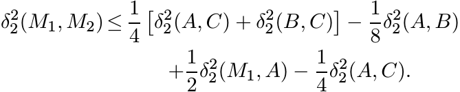
Since δ2(M1, A) = δ2(A, B)/2, the right-hand side of this inequality reduces to ![]() .
This proves (6.17). ■
.
This proves (6.17). ■
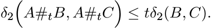
The inequality (6.17) can be used to prove a more general version of itself. For 0 ≤ t ≤ 1 let
 (6.18)
This is another notation for the geodesic curve γ(t) in (6.11). When t = 1/2 this is the geometric mean A#B. The more general version is in the following.
6.1.11 Corollary
Given four points B, C, B′, and C′ in Pn let
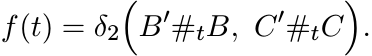
Then f is convex on [0, 1]; i.e.,
Proof. Since f is continuous it is sufficient to prove that it is midpoint-convex. Let M1 = B′#B, M2 = C′#C, and M = B′#C. By Proposition 6.1.10 we have δ2(M1, M) ≤ δ2(B, C)/2 and δ2(M, M2) ≤ δ2(B′, C′)/2. Hence

This shows that f is midpoint-convex. ■
Choosing B′ = C′ = A in (6.19) gives the following theorem called the convexity of the metric δ2.
6.1.12 Theorem
Let A, B and C be any three points in Pn. Then for all t in [0, 1] we have
 (6.20)
6.1.13 Exercise
For a fixed A in ![]() let f be the function
let f be the function ![]() . Show that if
. Show that if ![]() , then for 0 < t < 1
, then for 0 < t < 1
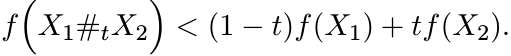 (6.21)
This is expressed by saying that the function f is strictly convex on ![]() . [Hint: Show
this for t = 1/2 first.]
. [Hint: Show
this for t = 1/2 first.]
6.2 THE METRIC SPACE 
In this section we briefly study some properties of the metric space ![]() with special
emphasis on convex sets.
with special
emphasis on convex sets.
6.2.1 Lemma
The exponential is a continuous map from the space ![]() onto the space
onto the space ![]() .
.
Proof. Let Hm be a sequence in ![]() converging to H. Then e−HmeH converges to I in the
metric induced by ||.||2. So all the eigenvalues
converging to H. Then e−HmeH converges to I in the
metric induced by ||.||2. So all the eigenvalues ![]() , 1 ≤ i ≤ n, converge to 1. The
relation (6.14) then shows that
, 1 ≤ i ≤ n, converge to 1. The
relation (6.14) then shows that ![]() goes to zero as m goes to ∞. ■
goes to zero as m goes to ∞. ■
6.2.2 Proposition
The metric space ![]() is complete.
is complete.
Proof. Let {Am} be a Cauchy sequence in ![]() and let Hm = log Am. By the EMI (6.8) {Hm}
is a Cauchy sequence in
and let Hm = log Am. By the EMI (6.8) {Hm}
is a Cauchy sequence in ![]() , and hence it converges to some H in
, and hence it converges to some H in ![]() . By Lemma 6.2.1 the
sequence {Am} converges to A = eH in the space
. By Lemma 6.2.1 the
sequence {Am} converges to A = eH in the space ![]() . ■
. ■
Note that Pn is not a complete subspace of ![]() . There it has a boundary consisting of
singular positive matrices. In terms of the metric δ2 these are “points at infinity.”
The next proposition shows that we may approach these points along geodesics. We
use A#tB for the matrix defined by (6.18) for every real t. When A and B commute,
this reduces to A1−tBt.
. There it has a boundary consisting of
singular positive matrices. In terms of the metric δ2 these are “points at infinity.”
The next proposition shows that we may approach these points along geodesics. We
use A#tB for the matrix defined by (6.18) for every real t. When A and B commute,
this reduces to A1−tBt.
6.2.3 Proposition
Let S be a singular positive matrix. Then there exist commuting elements A and B
in ![]() such that
such that

as t → ∞.
Proof. Apply a unitary conjugation and assume S = diag (λ1, . . . , λn) where λk are nonnegative for 1 ≤ k ≤ n, and λk = 0 for some k. If λk > 0, then put αk = βk = λk, and if λk = 0, then put αk = 1 and βk = 1/2. Let A = diag (α1, . . . , αn) and B = diag (β1, . . . , βn). Then
For the metric δ2 we have
and this goes to ∞ as t → ∞. ■
The point of the proposition is that the curve A#tB starts at A when t = 0, and “goes
away to infinity” in the metric space ![]() while converging to S in the space
while converging to S in the space ![]() .
.
It is conventional to extend some matrix operations from strictly positive matrices to singular positive matrices by taking limits. For example, the geometric mean A#B is defined by (4.10) for strictly positive matrices A and B, and then defined for singular positive matrices A and B as
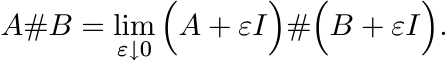
The next exercise points to the need for some caution when using this idea.
6.2.4 Exercise
The geometric mean A#B is continuous on pairs of strictly positive matrices, but is not so when extended to positive semidefinite matrices. (See Exercise 4.1.6.)
We have seen that any two points A and B in ![]() can be joined by a geodesic segment
[A, B] lying in
can be joined by a geodesic segment
[A, B] lying in ![]() . We say a subset
. We say a subset ![]() of
of ![]() is convex if for each pair of points A and
B in
is convex if for each pair of points A and
B in ![]() the segment [A, B] lies entirely in
the segment [A, B] lies entirely in ![]() . If
. If ![]() is any subset of
is any subset of ![]() , then the convex
hull of
, then the convex
hull of ![]() is the smallest convex set containing
is the smallest convex set containing ![]() . This set, denoted as conv
. This set, denoted as conv ![]() is the
intersection of all convex sets that contain
is the
intersection of all convex sets that contain ![]() . Clearly, the convex hull of any two
point set {A, B} is [A, B].
. Clearly, the convex hull of any two
point set {A, B} is [A, B].
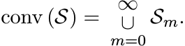
6.2.5 Exercise
Let S be any set in ![]() . Define inductively the sets
. Define inductively the sets ![]() as
as ![]() and
and
Show that
The next theorem says that if ![]() is a closed convex set in
is a closed convex set in ![]() , then a metric projection
onto
, then a metric projection
onto ![]() exists just as it does in a Hilbert space.
exists just as it does in a Hilbert space.
6.2.6 Theorem
Let ![]() be a closed convex set in
be a closed convex set in ![]() . Then for each
. Then for each ![]() there exists a point
there exists a point ![]() such that δ2(A,
C) < δ2(A, K) for every K in
such that δ2(A,
C) < δ2(A, K) for every K in ![]() ,
, ![]() . (In other words C is the unique best approximant
to A from the set
. (In other words C is the unique best approximant
to A from the set ![]() .)
.)
Proof. Let µ = inf {δ2(A, K) : K ∈ ![]() } . Then there exists a sequence {Cn} in
} . Then there exists a sequence {Cn} in ![]() such
that δ2(A, Cn) → µ. Given n and m, let M be the midpoint of the geodesic segment
[Cn, Cm]; i.e., M = Cn#Cm. By the convexity of
such
that δ2(A, Cn) → µ. Given n and m, let M be the midpoint of the geodesic segment
[Cn, Cm]; i.e., M = Cn#Cm. By the convexity of ![]() the point M is in
the point M is in ![]() . Using the semiparallelogram
law (6.16) we get
. Using the semiparallelogram
law (6.16) we get
and hence
As n and m go to ∞, the right-hand side of (6.22) goes to zero. Hence {Cn} is a Cauchy
sequence, and by Proposition 6.2.2 it converges to a limit C in ![]() . Since
. Since ![]() is closed,
C is in
is closed,
C is in ![]() . Further δ2(A, C) = lim δ2(A, Cn) = µ. If K is any other element of
. Further δ2(A, C) = lim δ2(A, Cn) = µ. If K is any other element of ![]() such
that δ2(A, K) = µ, then putting Cn = C and Cm = K in (6.22) we see that δ2(C, K)
= 0; i.e., C = K. ■
such
that δ2(A, K) = µ, then putting Cn = C and Cm = K in (6.22) we see that δ2(C, K)
= 0; i.e., C = K. ■
The map π(A) = C given by Proposition 6.2.6 may be called the metric projection onto K.
6.2.7 Theorem
Let π be the metric projection onto a closed convex set ![]() of
of ![]() . If A is any point of
. If A is any point of
![]() and π(A) = C, then for any D in
and π(A) = C, then for any D in ![]()
Proof. Let {Mn} be the sequence defined inductively as M0 = D, and Mn+1 = Mn#C. Then δ2(C, Mn) = 2−nδ2(C, D), and Mn converges to C = M∞. By the semiparallelogram law (6.16)

Hence,

Summing these inequalities we have
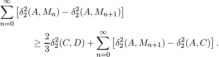
It is easy to see that the two series are absolutely convergent.
Let ![]() . Then the last inequality can be written as
. Then the last inequality can be written as
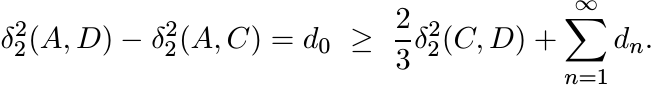
The same argument applied to Mn in place of D shows
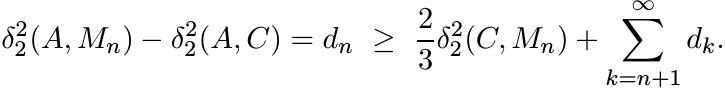
Thus
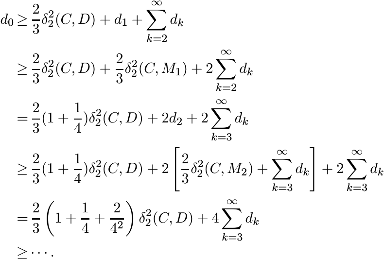
Since ![]() is convex, each
is convex, each ![]() , and hence dn ≥ 0. Thus we have
, and hence dn ≥ 0. Thus we have
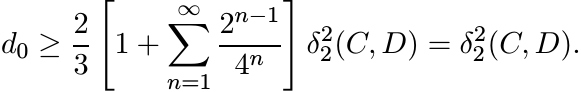
This proves the inequality (6.23). ■
6.2.8 The geometric mean once again
If ![]() is a Euclidean space with metric d, and a, b are any two points of
is a Euclidean space with metric d, and a, b are any two points of ![]() , then the
function
, then the
function
attains its minimum on ![]() at the unique point
at the unique point ![]() . In the metric space
. In the metric space ![]() this role is played
by the geometric mean.
this role is played
by the geometric mean.
Proposition. Let A and B be any two points of Pn, and let
Then the function f is strictly convex on ![]() , and has a unique minimum at the point
X0 = A#B.
, and has a unique minimum at the point
X0 = A#B.
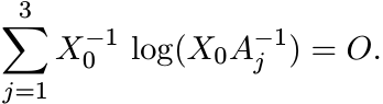
Proof. The strict convexity is a consequence of Exercise 6.1.13. The semiparallelogram law implies that for every X we have

Hence
This shows that f has a unique minimum at the point X0 = A#B. ■
6.3 CENTER OF MASS AND GEOMETRIC MEAN
In Chapter 4 we discussed, and resolved, the problems associated with defining a good geometric mean of two positive matrices. In this section we consider the question of a suitable definition of a geometric mean of more than two matrices. Our discussion will show that while the case of two matrices is very special, ideas that work for three matrices do work for more than three as well.
Given three positive matrices A1, A2, and A3, their geometric mean G(A1, A2, A3) should be a positive matrix with the following properties. If A1, A2, and A3 commute with each other, then G(A1A2A3) = (A1A2A3)1/3. As a function of its three variables, G should satisfy the conditions:
(i) G(A1, A2, A3) = G(Aπ(1), Aπ(2), Aπ(3)) for every permutation π of {1, 2, 3}.
(ii) G(A1, A2, A3) ≤ G(A′1, A2, A3) whenever A1 ≤ A′1.
(iii) G(X∗A1X, X∗A2X, X∗A3X) = X∗G(A1, A2, A3)X for all X ∈ GL(n).
(iv) G is continuous.
The first three conditions may be called symmetry, monotonicity, and congruence invariance, respectively.
None of the procedures that we used in Chapter 4 to define the geometric mean of two positive matrices extends readily to three. While two positive matrices can be diagonalized simultaneously by a congruence, in general three cannot be. The formula (4.10) has no obvious analogue for three matrices; nor does the extremal characterization (4.15). It is here that the connections with geometry made in Sections 6.1.7 and 6.2.8 suggest a way out: the geometric mean of three matrices should be the “center” of the triangle that has the three matrices as its vertices.
As motivation, consider the arithmetic mean of three points x1, x2, and x3 in a Euclidean
space ![]() . The point
. The point ![]() is characterized by several properties; three of them follow:
is characterized by several properties; three of them follow:
(i)
![]() is the unique point of intersection of the three medians of the triangle Δ(x1, x2,
x3). (This point is called the centroid of Δ.)
is the unique point of intersection of the three medians of the triangle Δ(x1, x2,
x3). (This point is called the centroid of Δ.)
(ii)
![]() is the unique point in
is the unique point in ![]() at which the function
at which the function
attains its minimum. (This point is the center of mass of the triple {x1, x2, x3} if each of them has equal mass.)
(iii)
![]() is the unique point of intersection of the nested sequence of triangles {Δn} in
which Δ1 = Δ(x1, x2, x3) and Δj+1 is the triangle whose vertices are the midpoints
of the three sides of Δj.
is the unique point of intersection of the nested sequence of triangles {Δn} in
which Δ1 = Δ(x1, x2, x3) and Δj+1 is the triangle whose vertices are the midpoints
of the three sides of Δj.
We may try to mimic these constructions in the space ![]() . As we will see, this has to
be done with some circumspection.
. As we will see, this has to
be done with some circumspection.
The first difficulty is with the identification of a triangle in this space. In Section
6.2 we defined convex hulls and observed that the convex hull of two points A1, A2
in ![]() is the geodesic segment [A1, A2]. It is harder to describe the convex hull of
three points A1, A2, A3. (This seems to be a difficult problem in Riemannian geometry.)
In the notation of Exercise 6.2.5, if
is the geodesic segment [A1, A2]. It is harder to describe the convex hull of
three points A1, A2, A3. (This seems to be a difficult problem in Riemannian geometry.)
In the notation of Exercise 6.2.5, if ![]() = {A1, A2, A3}, then
= {A1, A2, A3}, then ![]() = [A1, A2] ∪ [A2, A3]
∪ [A3, A1] is the union of the three “edges.” However,
= [A1, A2] ∪ [A2, A3]
∪ [A3, A1] is the union of the three “edges.” However, ![]() is not in general a “surface,”
but a “fatter” object. Thus it may happen that the three “medians” [A1, A2#A3], [A2,
A1#A3], and [A3, A1#A2] do not intersect at all in most cases. So, we have to abandon
this as a possible definition of the centroid of the triangle Δ(A1, A2, A3).
is not in general a “surface,”
but a “fatter” object. Thus it may happen that the three “medians” [A1, A2#A3], [A2,
A1#A3], and [A3, A1#A2] do not intersect at all in most cases. So, we have to abandon
this as a possible definition of the centroid of the triangle Δ(A1, A2, A3).
Next we ask whether for every triple of points A1, A2, A3 in ![]() there exists a (unique)
point X0 at which the function
there exists a (unique)
point X0 at which the function
attains its minimum value on ![]() . A simple argument using the semiparallelogram law
shows that such a point exists. This goes as follows.
. A simple argument using the semiparallelogram law
shows that such a point exists. This goes as follows.
Let m = inf f(X) and let {Xr} be a sequence in ![]() such that f(Xr) → m. By the semiparallellgram
law we have for j = 1, 2, 3, and for all r and s
such that f(Xr) → m. By the semiparallellgram
law we have for j = 1, 2, 3, and for all r and s

Summing up these three inequalities over j, we obtain

This shows that
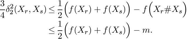
It follows that {Xr} is a Cauchy sequence, and hence it converges to a limit X0. Clearly f attains its minimum at X0. By Exercise 6.1.13 the function f is strictly convex and its minimum is attained at a unique point.
We define the “center of mass” of {A1, A2, A3} as the point
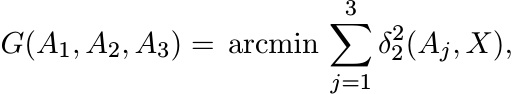 (6.24)
where the notation arcmin f(X) stands for the point X0 at which the function f(X)
attains its minimum value. It is clear from the definition that G(A1, A2, A3) is
a symmetric and continuous function of the three variables. Since each congruence
transformation ΓX is an isometry of ![]() it is easy to see that G is congruence invariant;
i.e.,
it is easy to see that G is congruence invariant;
i.e.,
Thus G has three of the four desirable properties listed for a good geometric mean at the beginning of this section. We do not know whether G is monotone. Some more properties of G are derived below.
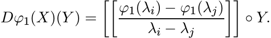
6.3.1 Lemma
Let φ1, φ2 be continuously differentiable real-valued functions on the interval (0, ∞) and let

for all ![]() . Then the derivative of h is given by the formula
. Then the derivative of h is given by the formula

Proof. By the product rule for differentiation (see MA, p. 312) we have

Choose an orthonormal basis in which X = diag (λ1, . . . , λn). Then by (2.40)
Hence,
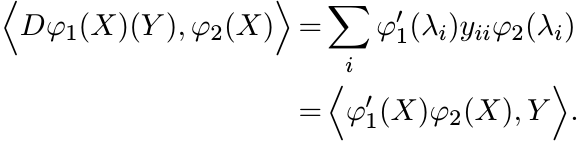
Similarly,

This proves the lemma. ■
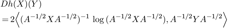
6.3.2 Corollary
Let ![]() ,
, ![]() . Then
. Then

We need a slight modification of this result. If
then
 (6.25)
for all ![]() .
.
6.3.3 Theorem
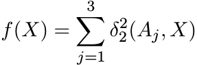
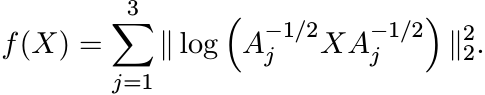
Let A1, A2, A3 be any three elements of ![]() , and let
, and let
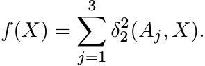 (6.26)
Then the derivative of f at X is given by
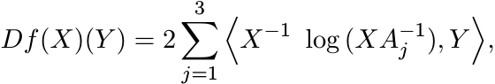 (6.27)
for all ![]() .
.
Proof. Using the relation (6.13) we have
Using (6.25) we see that Df(X)(Y ) is a sum of three terms of the form
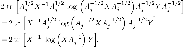
Here we have used the similarity invariance of trace at the first step, and then the relation
at the second step. The latter is valid for all matrices T with no eigenvalues on the half-line (−∞, 0] and for all invertible matrices S, and follows from the usual functional calculus. This proves the theorem. ■
6.3.4 Theorem
Let A1, A2, A3 be three positive matrices and let X0 = G(A1, A2, A3) be the point defined by (6.24). Then X0 is the unique positive solution of the equation
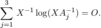 (6.28)
Proof. The point X0 is the unique minimum of the function (6.26),
and hence, is characterised by the vanishing of the derivative (6.27) for all ![]() . But
any matrix orthogonal to all Hermitian matrices is zero. Hence
. But
any matrix orthogonal to all Hermitian matrices is zero. Hence
 (6.29)
In other words X0 satisfies the equation (6.28). ■
6.3.5 Exercise
Let A1, A2, A3 be pairwise commuting positive matrices. Show that G(A1, A2, A3) = (A1A2A3)1/3.
6.3.6 Exercise
Let X and A be positive matrices. Show that
 (6.30)
(This shows that the matrices occurring in (6.29) are Hermitian.)
6.3.7 Exercise
Let w = (w1, w2, w3), where wj ≥ 0 and ![]() . We say that w is a set of weights. Let
. We say that w is a set of weights. Let
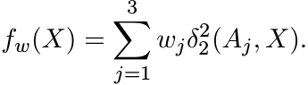
Show that fw is strictly convex, and attains a minimum at a unique point.
Let Gw(A1, A2, A3) be the point where fw attains its minimum. The special choice w = (1/3, 1/3, 1/3) leads to G(A1, A2, A3).
6.3.8 Proposition
Each of the points Gw(A1, A2, A3) lies in the closure of the convex hull conv ({A1, A2, A3}).
Proof. Let ![]() be the closure of conv ({A1, A2, A3}) and let π be the metric projection
onto
be the closure of conv ({A1, A2, A3}) and let π be the metric projection
onto ![]() . Then by Theorem 6.2.7,
. Then by Theorem 6.2.7, ![]()
![]() for every
for every ![]() . Hence fw(X) ≥ fw(π(X)) for all X. Thus
the minimum value of fw(X) cannot be attained at a point outside
. Hence fw(X) ≥ fw(π(X)) for all X. Thus
the minimum value of fw(X) cannot be attained at a point outside ![]() . ■
. ■
Now we turn to another possible definition of the geometric mean of three matrices inspired by the characterisation of the centre of a triangle as the intersection of a sequence of nested triangles.
Given A1, A2, A3 in ![]() inductively construct a sequence of triples
inductively construct a sequence of triples ![]() as follows. Set
as follows. Set
![]() , and let
, and let
6.3.9 Theorem
Let A1, A2, A3 be any three points in ![]() , and let
, and let ![]() be the sequence defined by (6.31).
Then for any choice of Xm in conv
be the sequence defined by (6.31).
Then for any choice of Xm in conv![]() the sequence {Xm} converges to a point X ∈ conv
({A1, A2, A3}). The point X does not depend on the choice of Xm.
the sequence {Xm} converges to a point X ∈ conv
({A1, A2, A3}). The point X does not depend on the choice of Xm.
Proof. The diameter of a set ![]() in
in ![]() is defined as
is defined as
It is easy to see, using convexity of the metric δ2, that if diam ![]() = M, then diam
= M, then diam
![]() .
.
Let ![]() . By (6.17), and what we said above, diam
. By (6.17), and what we said above, diam ![]() , where M0 = diam {A1, A2, A3}. The
sequence
, where M0 = diam {A1, A2, A3}. The
sequence ![]() is a decreasing sequence. Hence {Xm} is Cauchy and converges to a limit
X. Since Xm is in
is a decreasing sequence. Hence {Xm} is Cauchy and converges to a limit
X. Since Xm is in ![]() for all m, the limit X is in the closure of
for all m, the limit X is in the closure of ![]() . The limit is unique
as any two such sequences can be interlaced. ■
. The limit is unique
as any two such sequences can be interlaced. ■
6.3.10 A geometric mean of three matrices
Let G#(A1, A2, A3) be the limit point X whose existence has been proved in Theorem 6.3.9. This may be thought of as a geometric mean of A1, A2, A3. From its construction it is clear that G# is a symmetric continuous function of A1, A2, A3. Since the geometric mean A#B of two matrices is monotone in A and B and is invariant under congruence transformations, these properties are inherited by G#(A1, A2, A3) as its construction involves successive two-variable means and limits.
Exercise Show that for a commuting triple A1, A2, A3 of positive matrices G#(A1, A2, A3) = (A1A2A3)1/3.
One may wonder whether G#(A1, A2, A3) is equal to the centre of mass G(A1, A2, A3). It turns out that this is not always the case. Thus we have here two different candidates for a geometric mean of three matrices. While G# has all properties that we seek, it is not known whether G is monotone in its arguments. It does have all other desired properties.
6.4 RELATED INEQUALITIES
Some of the inequalities proved in Section 6.1 can be generalized from the special ||·||2 norm to all Schatten ||·||p norms and to the larger class of unitarily invariant norms. These inequalities are very closely related to others proved in very different contexts like quantum statistical mechanics. This section is a brief indication of these connections.
Two results from earlier chapters provide the basis for our generalizations. In Exercise 2.7.12 we saw that for a positive matrix A
for every X and every unitarily invariant norm. In Section 5.2.9 we showed that for every choice of n positive numbers λ1, . . . , λn, the matrix
is positive. Using these we can easily prove the following generalized version of Proposition 6.1.2.
6.4.1 Proposition (Generalized IEMI)
For all H and K in Hn we have
for every unitarily invariant norm.
In the definition (6.2) replace || · ||2 by any unitarily invariant norm ||| · ||| and call the resulting length L|||·|||; i.e.,
 (6.33)
Since |||X||| is a (symmetric gauge) function of the singular values of X, Lemma 6.1.1 carries over to L|||·|||. The analogue of (6.4),
is a metric on ![]() invariant under congruence transformations. The generalized IEMI
leads to a generalized EMI. For all A, B in
invariant under congruence transformations. The generalized IEMI
leads to a generalized EMI. For all A, B in ![]() we have
we have
or, in other words, for all H, K in ![]()
Some care is needed while formulating statements about uniqueness of geodesics. Many
unitarily invariant norms have the property that, in the metric they induce on ![]() ,
the straight line segment is the unique geodesic joining any two given points. If
a norm ||| · ||| has this property, then the metric δ|||·||| on
,
the straight line segment is the unique geodesic joining any two given points. If
a norm ||| · ||| has this property, then the metric δ|||·||| on ![]() inherits it. The
Schatten p-norms have this property for 1 < p < ∞, but not for p = 1 or ∞.
With this proviso, statements made in Sections 6.1.5 and 6.1.6 can be proved in the
more general setting. In particular, we have
inherits it. The
Schatten p-norms have this property for 1 < p < ∞, but not for p = 1 or ∞.
With this proviso, statements made in Sections 6.1.5 and 6.1.6 can be proved in the
more general setting. In particular, we have
The geometric mean A#B defined by (4.10) is equidistant from A and B in each of the metrics δ|||·|||. For certain metrics, such as the ones corresponding to Schatten p-norms for 1 < p < ∞, this is the unique “metric midpoint” between A and B.
The parallelogram law and the semiparallelogram law, however, characterize a Hilbert space norm and the associated Riemannian metric. These are not valid for other metrics.
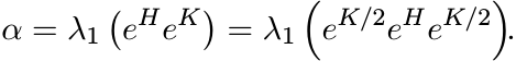
Now we can see the connection between these inequalities arising from geometry to others related to physics. Some facts about majorization and unitarily invariant norms are needed in the ensuing discussion. Let H, K be Hermitian matrices. From (6.36) and (6.37) we have
The exponential function is convex and monotonically increasing on ![]() . Such functions
preserve weak majorization (Corollary II.3.4 in MA). Using this property we obtain
from the inequality (6.38)
. Such functions
preserve weak majorization (Corollary II.3.4 in MA). Using this property we obtain
from the inequality (6.38)
Two special cases of this are well-known inequalities in physics. The special cases of the || · ||1 and the || · || norms in (6.39) say
and
where λ1(X) is the largest eigenvalue of a matrix with real eigenvalues. The first of these is called the Golden-Thompson inequality and the second is called Segal’s inequality.
The inequality (6.41) can be easily derived from the operator monotonicity of the logarithm function (Exercise 4.2.5 and Section 5.3.7).
Let
Then
and hence
Since log is an operator monotone function on (0, ∞), it follows that
Hence
and therefore
This leads to (6.41).
More interrelations between various inequalities are given in the next section and in the notes at the end of the chapter.
6.5 SUPPLEMENTARY RESULTS AND EXERCISES
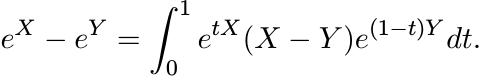
The crucial inequality (6.6) has a short alternate proof based on the inequality between the geometric and the logarithmic means. This relies on the following interesting formula for the derivative of the exponential map:
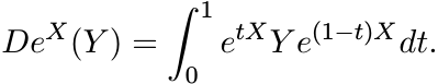 (6.42)
This formula, attributed variously to Duhamel, Dyson, Feynman, and Schwinger, has an easy proof. Since
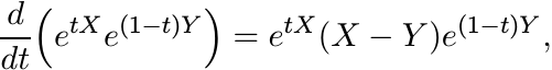
we have
Hence
This is exactly the statement (6.42).
Now let H and K be Hermitian matrices. Using the identity
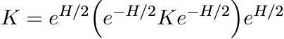
and the first inequality in (5.34) we obtain
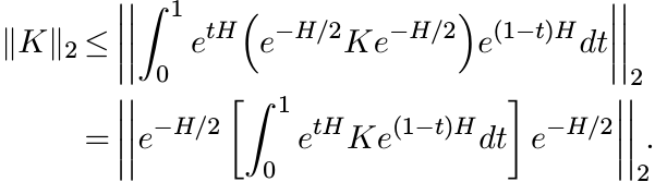
The last integral is equal to DeH(K). Hence,
This is the IEMI (6.6).
The inequality (5.35) generalizes (5.34) to all unitarily invariant norms. So, exactly the same argument as above leads to a proof of (6.32) as well.
From the expression (6.14) it is clear that
for all ![]() . Similarly, from (6.37) we see that
. Similarly, from (6.37) we see that
An important notion in geometry is that of a Riemannian symmetric space. By definition, this is a connected Riemannian manifold M for each point p of which there is an isometry σp of M with two properties:
(i) σp(p) = p, and
(ii) the derivative of σp at p is multiplication by −1.
The space ![]() is a Riemannian symmetric space. We show this using the notation and some
basic facts on matrix differential calculus from Section X.4 of MA. For each
is a Riemannian symmetric space. We show this using the notation and some
basic facts on matrix differential calculus from Section X.4 of MA. For each ![]() let
σA be the map defined on
let
σA be the map defined on ![]() by
by
Clearly σA(A) = A. Let ![]() be the inversion map. Then σA is the composite
be the inversion map. Then σA is the composite ![]() . The derivative
of
. The derivative
of ![]() is given by
is given by ![]() −X−1Y X−1, while ΓA being a linear map is equal to its own derivative.
So, by the chain rule
−X−1Y X−1, while ΓA being a linear map is equal to its own derivative.
So, by the chain rule
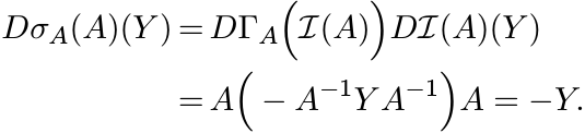
Thus Dσp(A) is multiplication by −1.
The Riemannian manifold ![]() has nonpositive curvature. The EMI captures the essence
of this fact. We explain this briefly.
has nonpositive curvature. The EMI captures the essence
of this fact. We explain this briefly.
Consider a triangle Δ(O, H, K) with vertices O, H, and K in ![]() . The image of this set
under the exponential map is a “triangle” Δ(I, eH, eK) in
. The image of this set
under the exponential map is a “triangle” Δ(I, eH, eK) in ![]() . By Proposition 6.1.5
the δ2-lengths of the sides [I, eH] and [I, eK] are equal to the || · ||2 -lengths
of the sides [O, H] and [O, K], respectively. By the EMI (6.8) the third side [eH,
eK] is longer than [H, K]. Keep the vertex O as a fixed pivot and move the sides
[O, H] and [O, K] apart to get a triangle Δ(O, H′, K′) in
. By Proposition 6.1.5
the δ2-lengths of the sides [I, eH] and [I, eK] are equal to the || · ||2 -lengths
of the sides [O, H] and [O, K], respectively. By the EMI (6.8) the third side [eH,
eK] is longer than [H, K]. Keep the vertex O as a fixed pivot and move the sides
[O, H] and [O, K] apart to get a triangle Δ(O, H′, K′) in ![]() whose three sides now
have the same lengths as the δ2-lengths of the sides of Δ(I, eH, eK) in
whose three sides now
have the same lengths as the δ2-lengths of the sides of Δ(I, eH, eK) in ![]() . Such a
triangle is called a comparison triangle for Δ(I, eH, eK) and it is unique up to
an isometry of
. Such a
triangle is called a comparison triangle for Δ(I, eH, eK) and it is unique up to
an isometry of ![]() . The fact that the comparison triangle in the Euclidean space
. The fact that the comparison triangle in the Euclidean space ![]() is
“fatter” than the triangle Δ(I, eH, eK) is a characterization of a space of nonpositive
curvature.
is
“fatter” than the triangle Δ(I, eH, eK) is a characterization of a space of nonpositive
curvature.
It may be instructive here to compare the situation with the space ![]() consisting of
unitary matrices. This is a compact manifold of nonnegative curvature. In this case
the real vector space
consisting of
unitary matrices. This is a compact manifold of nonnegative curvature. In this case
the real vector space ![]() consisting of skew-Hermitian matrices is mapped by the exponential
onto
consisting of skew-Hermitian matrices is mapped by the exponential
onto ![]() . The map is not injective in this case; it is a local diffeomorphism.
. The map is not injective in this case; it is a local diffeomorphism.
6.5.1 Exercise
Let H and K be any two skew-Hermitian matrices. Show that
[Hint: Follow the steps in the proof of Proposition 6.1.2. Now the λi are imaginary. So the hyperbolic function sinh occurring in the proof of Proposition 6.1.2 is replaced by the circular function sin. Alternately prove this using the formula (6.42). Observe that etH is unitary.]
As a consequence we have the opposite of the inequality (6.8) in this case: if A
and B are sufficiently close in ![]() , then
, then
Thus the exponential map decreases distance locally. This fact captures the nonnegative
curvature of ![]() .
.
Of late there has been interest in general metric spaces of nonpositive curvature
(not necessarily Riemannian manifolds). An important consequence of the generalised
EMI proved in Section 6.4 is that for every unitarily invariant norm the space ![]() is
a metric space of nonpositive curvature. These are examples of Finsler manifolds,
where the metric arises from a non-Euclidean metric on the tangent space.
is
a metric space of nonpositive curvature. These are examples of Finsler manifolds,
where the metric arises from a non-Euclidean metric on the tangent space.
A metric space (X, d) is said to satisfy the semiparallelogram law if for any two points a, b ∈ X, there exists a point m such that
for all c ∈ X.
6.5.2 Exercise
Let (X, d) be a metric space with the semiparallelogram law. Show that the point
m arising in the definition is unique and is the metric midpoint of a and b; i.e.,
m is the point at which d(a, m) = d(b, m) = ![]() .
.
A complete metric space satisfying the semiparallelogram law is called a Bruhat-Tits
space. We have shown that ![]() is such a space. Those of our proofs that involved only
completeness and the semiparallelogram law are valid for all Bruhat-Tits spaces.
See, for example, Theorems 6.2.6 and 6.2.7.
is such a space. Those of our proofs that involved only
completeness and the semiparallelogram law are valid for all Bruhat-Tits spaces.
See, for example, Theorems 6.2.6 and 6.2.7.
In the next two exercises we point out more connections between classical matrix inequalities and geometric facts of this chapter. We use the notation of majorization and facts about unitarily invariant norms from MA, Chapters II and IV. The reader unfamiliar with these may skip this part.
6.5.3 Exercise
An inequality due to Gel’fand, Naimark, and Lidskii gives relations between eigenvalues of two positive matrices A and B and their product AB. This says
log λ↓(A) + log λ↑(B) ≺ log λ(AB) ≺ log λ↓(A) + log λ↓(B). (6.47) See MA p. 73. Let A, B, and C be three positive matrices. Then
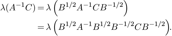
So, by the second part of (6.47)
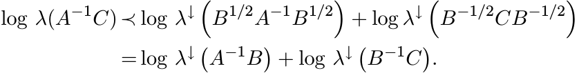
Use this to show directly that δ|||·||| defined by (6.36) is a metric on ![]() .
.
6.5.4 Exercise
Let A and B be positive. Then for 0 ≤ t ≤ 1 and 1 ≤ k ≤ n we have
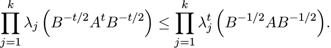 (6.48)
See MA p. 258. Take logarithms of both sides and use results on majorization to show that
This may be rewritten as
Show that this implies that the metric δ|||·||| is convex.
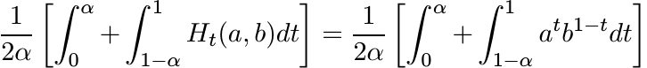
In Section 4.5 we outlined a general procedure for constructing matrix means from scalar means. Two such means are germane to our present discussion. The function f in (4.69) corresponding to the logarithmic mean is
So the logarithmic mean of two positive matrices A and B given by the formula (4.71) is
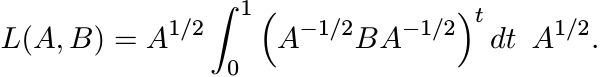
In other words
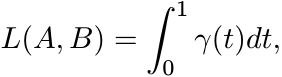 (6.49)
where γ(t) is the geodesic segment joining A and B.
Likewise, for 0 ≤ t ≤ 1 the Heinz mean
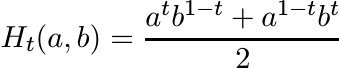 (6.50)
leads to the function
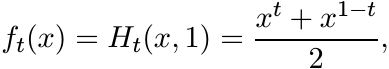
and then to the matrix Heinz mean
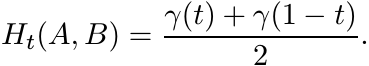 (6.51)
The following theorem shows that the geodesic γ(t) has very intimate connections with the order relation on Pn.
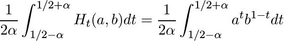
6.5.5 Theorem
For every α in [0, 1/2] we have
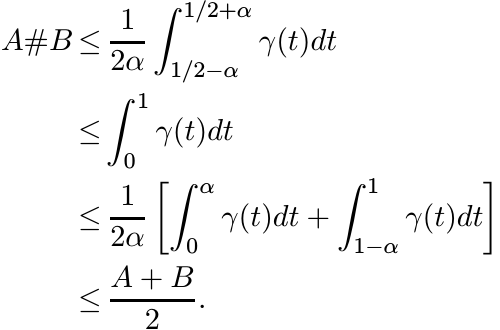
Proof. It is enough to prove the scalar versions of these inequalities as they are preserved in the transition to matrices by our construction. For fixed a and b, Ht(a, b) is a convex function of t on [0, 1]. It is symmetric about the point t = 1/2 at which it attains its minimum. Hence the quantity
is an increasing function of α for 0 ≤ α ≤ 1/2. Similarly,
is a decreasing function of α. These considerations show
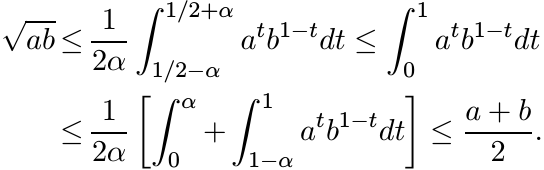
The theorem follows from this. ■
6.5.6 Exercise
Show that for 0 ≤ t ≤ 1
[Hint: Show that for each λ > 0 we have λt ≤ (1 − t) + tλ.]
6.5.7 Exercise
Let Φ be any positive linear map on ![]() . Then for all positive matrices A and B
. Then for all positive matrices A and B
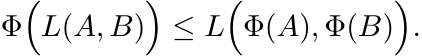
[Hint: Use Theorem 4.1.5 (ii).]
6.5.8 Exercise
The aim of this exercise is to give a simple proof of the convergence argument needed to establish the existence of G#(A1, A2, A3) defined in Section 6.3.10.
(i) Assume that A1 ≤ A2 ≤ A3. Then the sequences defined in (6.31) satisfy
The sequence ![]() is increasing and
is increasing and ![]() is decreasing. Hence the limits
is decreasing. Hence the limits
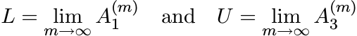
exist. Show that L = U. Thus
Call this limit G#(A1, A2, A3).
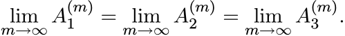
(ii) Now let A1, A2, A3 be any three positive matrices. Choose positive numbers λ and µ such that
Let (B1, B2, B3) = (A1, λA2, µA3). Apply the special case (i) to get the limit G#(B1, B2, B3). The same recursion applied to the triple of numbers (a1, a2, a3) = (1, λ, µ) gives
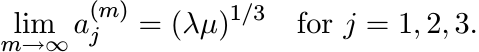
Since
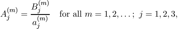
it follows that the sequences ![]() , j = 1, 2, 3, converge to the limit G#(B1, B2, B3)/(λµ)1/3.
, j = 1, 2, 3, converge to the limit G#(B1, B2, B3)/(λµ)1/3.
6.5.9 Exercise
Show that the center of mass defined by (6.24) has the property
for all positive matrices A1, A2, A3. Show that G# also satisfies this relation.
6.6 NOTES AND REFERENCES
Much of the material in Sections 6.1 and 6.2 consists of standard topics in Riemannian geometry. The arrangement of topics, the emphasis, and some proofs are perhaps eccentric. Our view is directed toward applications in matrix analysis, and the treatment may provide a quick introduction to some of the concepts. The entire chapter is based on R. Bhatia and J. A. R. Holbrook, Riemannian geometry and matrix geometric means, Linear Algebra Appl., 413 (2006) 594–618.
Two books on Riemannian geometry that we recommend are M. Berger, A Panoramic View
of Riemannian Geometry, Springer, 2003, and S. Lang, Fundamentals of Differential
Geometry, Springer, 1999. Closely related to our discussion is M. Bridson and A.
Haefliger, Metric Spaces of Non-positive Curvature, Springer, 1999. Most of the
texts on geometry emphasize group structures and seem to downplay the role of the
matrices that constitute these groups. Lang’s text is exceptional in this respect.
The book A. Terras, Harmonic Analysis on Symmetric Spaces and Applications II, Springer,
1988, devotes a long chapter to the space ![]() .
.
The proof of Proposition 6.1.2 is close to the treatment in Lang’s book. (Lang says he follows “Mostow’s very elegant exposition of Cartan’s work.”) The linear algebra in our proof looks neater because a part of the work has been done earlier in proving the Daleckii-Krein formula (2.40) for the derivative. The second proof given at the beginning of Section 6.5 is shorter and more elementary. This is taken from R. Bhatia, On the exponential metric increasing property, Linear Algebra Appl., 375 (2003) 211–220.
Explicit formulas like (6.11) describing geodesics are generally not emphasized in geometry texts. This expression has been used often in connection with means. With the notation A#tB this is called the t-power mean. See the comprehensive survey F. Hiai, Log-majorizations and norm inequalities for exponential operators, Banach Center Publications Vol. 38, pp. 119–181.
The role of the semiparallelogram law is highlighted in Chapter XI of Lang’s book. A historical note on page 313 of this book places it in context. To a reader oriented towards analysis in general, and inequalities in particular, this is especially attractive. The expository article by J. D. Lawson and Y. Lim, The geometric mean, matrices, metrics and more, Am. Math. Monthly, 108 (2001) 797–812, draws special attention to the geometry behind the geometric mean.
Problems related to convexity in differentiable manifolds are generally difficult. According to Note 6.1.3.1 on page 231 of Berger’s book the problem of identifying the convex hull of three points in a Riemannian manifold of dimension 3 or more is still unsolved. It is not even known whether this set is closed. This problem is reflected in some of our difficulties in Section 6.3.
Berger attributes to E. Cartan, Groupes simples clos et ouverts et géometrie Riemannienne,
J. Math. Pures Appl., 8 (1929) 1–33, the introduction of the idea of center of mass
in Riemannian geometry. Cartan showed that in a complete manifold of nonpositive
curvature (such as ![]() ) every compact set has a unique center of mass. He used this
to prove his fundamental theorem that says any two compact maximal subgroups of a
semisimple Lie group are always conjugate.
) every compact set has a unique center of mass. He used this
to prove his fundamental theorem that says any two compact maximal subgroups of a
semisimple Lie group are always conjugate.
The idea of using the center of mass to define a geometric mean of three positive matrices occurs in the paper of Bhatia and Holbrook cited earlier and in M. Moakher, A differential geometric approach to the geometric mean of symmetric positive-definite matrices, SIAM J. Matrix Anal. Appl., 26 (2005) 735–747. This paper contains many interesting ideas. In particular, Theorem 6.3.4 occurs here. Applications to problems of elasticity are discussed in M. Moakher, On the averaging of symmetric positive-definite tensors, preprint (2005).
The manifold ![]() is the most studied example of a manifold of nonpositive curvature.
However, one of its basic features—order—seems not to have received any attention.
Our discussion of the center of mass and Theorem 6.5.5 show that order properties
and geometric properties are strongly interlinked. A study of these properties should
lead to a better understanding of this manifold.
is the most studied example of a manifold of nonpositive curvature.
However, one of its basic features—order—seems not to have received any attention.
Our discussion of the center of mass and Theorem 6.5.5 show that order properties
and geometric properties are strongly interlinked. A study of these properties should
lead to a better understanding of this manifold.
The mean G#(A1, A2, A3) was introduced in T. Ando, C.-K Li, and R. Mathias, Geometric Means, Linear Algebra Appl., 385 (2004) 305–334. Many of its properties are derived in this paper which also contains a detailed survey of related matters. The connection with Riemannian geometry was made in the Bhatia-Holbrook paper cited earlier. That G# and the center of mass may be different, is a conclusion made on the basis of computer-assisted numerical calculations reported in Bhatia-Holbrook. A better theoretical understanding is yet to be found.
As explained in Section 6.5 the EMI reflects the fact that ![]() has nonpositive curvature.
Inequalities of this type are called CAT(0) inequalities; the initials C, A, T are
in honour of E. Cartan, A. D. Alexandrov, and A. Toponogov, respectively. These ideas
have been given prominence in the work of M. Gromov. See the book W. Ballmann, M.
Gromov, and V. Schroeder, Manifolds of Nonpositive Curvature, Birkhäuser, 1985,
and the book by Bridson and Haefliger cited earlier. A concept of curvature for metric
spaces (not necessarily Riemannian manifolds) is defined and studied in the latter.
The generalised EMI proved in Section 6.4 shows that the space
has nonpositive curvature.
Inequalities of this type are called CAT(0) inequalities; the initials C, A, T are
in honour of E. Cartan, A. D. Alexandrov, and A. Toponogov, respectively. These ideas
have been given prominence in the work of M. Gromov. See the book W. Ballmann, M.
Gromov, and V. Schroeder, Manifolds of Nonpositive Curvature, Birkhäuser, 1985,
and the book by Bridson and Haefliger cited earlier. A concept of curvature for metric
spaces (not necessarily Riemannian manifolds) is defined and studied in the latter.
The generalised EMI proved in Section 6.4 shows that the space ![]() with the metric
δ|||·||| is a metric space (a Finsler manifold) of nonpositive curvature.
with the metric
δ|||·||| is a metric space (a Finsler manifold) of nonpositive curvature.
Segal’s inequality was proved in I. Segal, Notes towards the construction of nonlinear relativistic quantum fields III, Bull. Am. Math. Soc., 75 (1969) 1390–1395. The simple proof given in Section 6.4 is borrowed from B. Simon, Trace Ideals and Their Applications, Second Edition, American Math. Society, 2005. The Golden-Thompson inequality is due to S. Golden, Lower bounds for the Helmholtz function, Phys. Rev. B, 137 (1965) 1127–1128, and C. J. Thompson, Inequality with applications in statistical mechanics, J. Math. Phys., 6 (1965) 1812–1813. Stronger versions and generalizations to other settings (like Lie groups) have been proved. Complementary inequalities have been proved by F. Hiai and D. Petz, The Golden-Thompson trace inequality is complemented, Linear Algebra Appl., 181 (1993) 153–185, and by T. Ando and F. Hiai, Log majorization and complementary Golden-Thompson type inequalities, ibid., 197/198 (1994) 113–131. These papers are especially interesting in our context as they involve the means A#tB in the formulation and the proofs of several results. The connection between means, geodesics, and inequalities has been explored in several interesting papers by G. Corach and coauthors. Illustrative of this work and especially close to our discussion are the two papers by G. Corach, H. Porta and L. Recht, Geodesics and operator means in the space of positive operators, Int. J. Math., 4 (1993) 193–202, and Convexity of the geodesic distance on spaces of positive operators, Illinois J. Math., 38 (1994) 87–94.
The logarithmic mean L(A, B) has not been studied before. The definition (6.49) raises interesting questions both for matrix theory and for geometry. In differential geometry it is common to integrate (real) functions along curves. Here we have the integral of the curve itself. Theorem 6.5.5 relates this object to other means, and includes the operator analogue of the inequality between the geometric, logarithmic, and arithmetic means. The norm version of this inequality appears as Proposition 3.2 in F. Hiai and H. Kosaki, Means for matrices and comparison of their norms, Indiana Univ. Math. J., 48 (1999) 899–936. Exercise 6.5.8 is based on the paper D. Petz and R. Temesi, Means of positive numbers and matrices, SIAM J. Matrix Anal. Appl., 27 (2005) 712–720.