
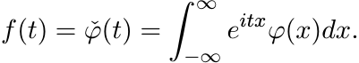
Chapter Five
Positive Definite Functions
Positive definite functions arise naturally in many areas of mathematics. In this chapter we study some of their basic properties, construct some examples, and use them to derive interesting results about positive matrices.
5.1 BASIC PROPERTIES
Positive definite sequences were introduced in Section 1.1.3. We repeat the definition.
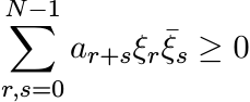
A (doubly infinite) sequence of complex numbers {an : n ∈ ![]() } is said to be positive
definite if for every positive integer N, we have
} is said to be positive
definite if for every positive integer N, we have
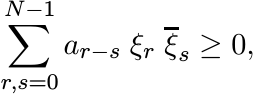 (5.1)
(5.1)for every finite sequence of complex numbers ξ0, ξ1, . . . , ξN−1. This condition is equivalent to the requirement that for each N = 1, 2, . . . , the N × N matrix
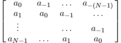 (5.2)
(5.2)is positive.
From this condition it is clear that we must have
A complex-valued function φ on ![]() is said to be positive definite if for every positive
integer N, we have
is said to be positive definite if for every positive
integer N, we have
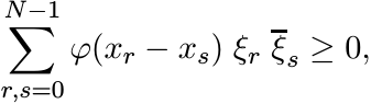 (5.4)
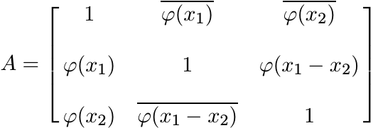
(5.4)for every choice of real numbers x0, x1, . . . , xN−1, and complex numbers ξ0, ξ1, . . . , ξN−1. In other words φ is positive definite if for each N = 1, 2, . . . the N × N matrix
is positive for every choice of real numbers x0, . . . , xN−1. It follows from this condition that
Thus every positive definite function is bounded, and its maximum absolute value is attained at 0.
5.1.1 Exercise
Let φ(x) be the characteristic function of the set ![]() ; i.e., φ(x) = 1 if
; i.e., φ(x) = 1 if ![]() and φ(x)
= 0 if
and φ(x)
= 0 if ![]() . Show that φ is positive definite. This remains true when
. Show that φ is positive definite. This remains true when ![]() is replaced by
any additive subgroup of
is replaced by
any additive subgroup of ![]() .
.
5.1.2 Lemma
If φ is positive definite, then for all x1, x2
Proof. Assume, without loss of generality, that φ(0) = 1. Choose x0 = 0. The 3 × 3 matrix
is positive. So for every vector u, the inner product ![]() . Choose u = (z, 1, −1) where
z is any complex number. This gives the inequality
. Choose u = (z, 1, −1) where
z is any complex number. This gives the inequality
Now choose ![]() . This gives
. This gives
Exercise 5.1.1 showed us that a positive definite function φ need not be continuous.
Lemma 5.1.2 shows that if the real part of φ is continuous at 0, then φ is continuous
everywhere on ![]() .
.
5.1.3 Exercise
Let φ(x) be positive definite. Then
(i)
![]() is positive definite.
is positive definite.
(ii) For every real number t the function φ(tx) is positive definite.
5.1.4 Exercise
(i) If φ1, φ2 are positive definite, then so is their product φ1φ2. (Schur’s theorem.)
(ii) If φ is positive definite, then |φ|2 is positive definite. So is Re φ.
5.1.5 Exercise
(i) If φ1, . . . , φn are positive definite, and a1, . . . , an are positive real numbers, then a1φ1 + · · · + anφn is positive definite.
(ii) If {φn} is a sequence of positive definite functions and φn(x) → φ(x) for all x, then φ is positive definite.
(iii)
If φ is positive definite, then eϕ is positive definite, and so is eϕ+a for every
![]() .
.
(iv)
If φ(x) is a measurable positive definite function and f(t) is a nonnegative integrable
function, then ![]() is positive definite.
is positive definite.
(v)
If µ is a finite positive Borel measure on ![]() and φ(x) a measurable positive definite
function, then the function
and φ(x) a measurable positive definite
function, then the function ![]() is positive definite. (The statement (iv) is a special
case of (v).)
is positive definite. (The statement (iv) is a special
case of (v).)
Let I be any interval and let K(x, y) be a bounded continuous complex-valued function on I × I. We say K is a positive definite kernel if
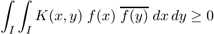 (5.7)
(5.7)for every continuous integrable function f on the interval I.
5.1.6 Exercise
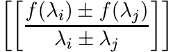
(i) A bounded continuous function K(x, y) on I × I is a positive definite kernel if and only if for all choices of points x1, . . . , xN in I, the N × N matrix [[K(xi, xj)]] is positive.
(ii)
A bounded continuous function φ on ![]() is positive definite if and only if the kernel
K(x, y) = φ(x − y) is positive definite.
is positive definite if and only if the kernel
K(x, y) = φ(x − y) is positive definite.
5.2 EXAMPLES
5.2.1
The function φ(x) = eix is positive definite since
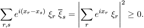
Exercise: Write the matrix (5.5) in this case as uu∗ where u is a column vector.
This example is fundamental. It is a remarkable fact that all positive definite functions can be built from this one function by procedures outlined in Section 5.1.
5.2.2
The function φ(x) = cos x is positive definite.
Exercise: sin x is not positive definite. The matrix A in Exercise 1.6.6 has entries aij = cos(xi − xj) where xi = 0, π/4, π/2, 3π/4. It follows that | cos x| is not positive definite.
5.2.3
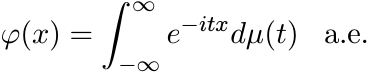
For each ![]() , φ(x) = eitx is a positive definite function.
, φ(x) = eitx is a positive definite function.
5.2.4
Let ![]() and let f(t) ≥ 0. Then
and let f(t) ≥ 0. Then
 (5.8)
(5.8)
is positive definite. More generally, if µ is a positive finite Borel measure on
![]() , then
, then
 (5.9)
(5.9)
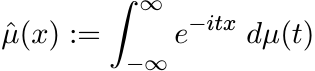
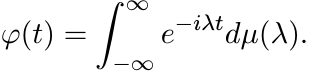
is positive definite. The function ![]() is called the Fourier transform of f and
is called the Fourier transform of f and ![]() is
called the Fourier-Stieltjes transform of µ. Both of them are bounded uniformly continuous
functions.
is
called the Fourier-Stieltjes transform of µ. Both of them are bounded uniformly continuous
functions.
These transforms give us many interesting positive definite functions.
5.2.5
One of the first calculations in probability theory is the computation of an integral:
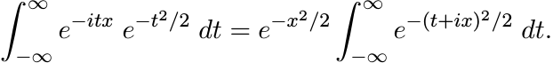
The integral on the right hand side can be evaluated using Cauchy’s theorem. Let C be the rectangular contour with vertices −R, R, R + ix, −R + ix. The integral of the analytic function f(z) = e−z2/2 along this contour is zero. As R → ∞, the integral along the two vertical sides of this contour goes to zero. Hence
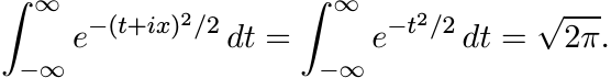
So,
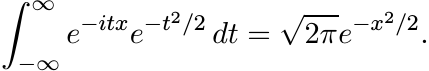 (5.10)
(This shows that, with a suitable normalization, the function e−x2/2 is its own Fourier transform.) Thus for each a ≥ 0, the function φ(x) = e−ax2 is positive definite.
5.2.6
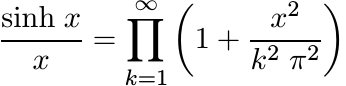
The function φ(x) = sin x/x is positive definite. To see this one can use the product formula
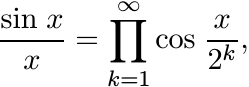 (5.11)
and observe that each of the factors in this infinite product is a positive definite function. Alternately, we can use the formula.
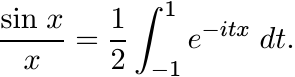 (5.12)
(This integral is the Fourier transform of the characteristic function ![]() .)
.)
We have tacitly assumed here that φ(0) = 1. This is natural. If we assign φ(0) any value larger than 1, the resulting (discontinuous) function is also positive definite.
5.2.7
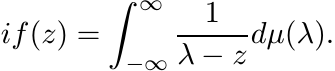
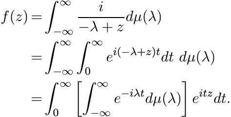
The integral
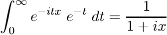
shows that the function φ(x) = 1/(1 + ix) is positive definite. The functions 1/(1 − ix) and 1/(1 + x2) are positive definite.
5.2.8
The integral formulas
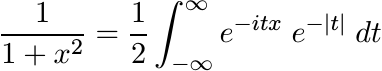
and
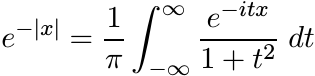
show that the functions 1/(1 + x2) and e−|x| are positive definite. (They are nonnegative and are, up to a constant factor, Fourier transforms of each other.)
5.2.9
From the product representations
 (5.13)
and
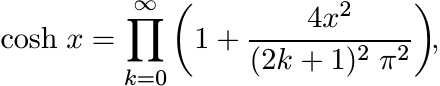 (5.14)
one sees (using the fact that 1/(1 + a2x2) is positive definite) that the functions x/(sinh x) and 1/(cosh x) are positive definite. (Contrast this with 5.2.6 and 5.2.2.)
5.2.10
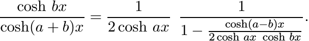
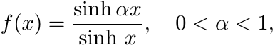
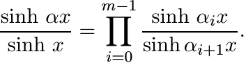
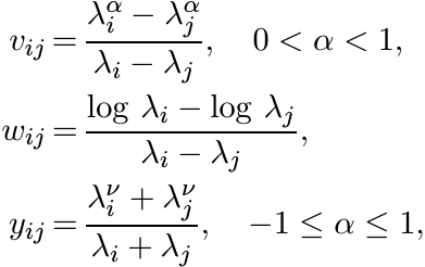
For 0 < α < 1, we have from (5.13)
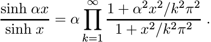 (5.15)
Each factor in this product is of the form
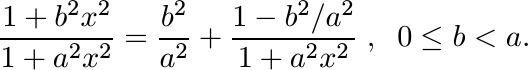
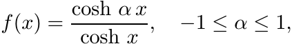
This shows that the function sinh αx/sinh x is positive definite for 0 ≤ α ≤ 1. In the same way using (5.14) one can see that cosh αx/cosh x is positive definite for −1 ≤ α ≤ 1. The function
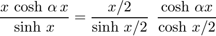
is positive definite for −1/2 ≤ α ≤ 1/2, as it is the product of two such functions.
5.2.11
The integral
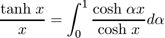
shows that tanh x/x is a positive definite function.
(Once again, it is natural to assign the functions sinh x/x, sinh αx/x and tanh x/x the values 1, α and 1, respectively, at x = 0. Then the functions under consideration are continuous and positive definite. Assigning them larger values at 0 destroys continuity but not positive definiteness.)
5.2.12
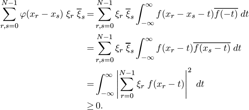
One more way of constructing positive definite functions is by convolutions of functions
in ![]() . For any function f let
. For any function f let ![]() be the function defined as
be the function defined as ![]() . If
. If ![]() then the function
then the function ![]() defined as
defined as
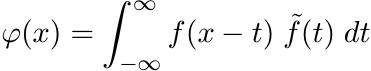
is a continuous function vanishing at ∞. It is a positive definite function since
5.2.13
Let R be a positive real number. The tent function (with base R) is defined as
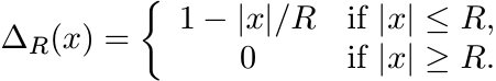 (5.16)
A calculation shows that
So, ∆R(x) is positive definite for all R > 0.
5.2.14
For R > 0, let δR be the continuous function defined as
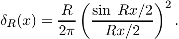 (5.17)
From 5.2.6 it follows that δR is positive definite. The family {δR}R>0 is called the Fejér kernel on R. It has the following properties (required of any “summability kernel” in Fourier analysis):
(i) δR(x) ≥ 0 for all x, and for all R > 0.
(ii) For every a > 0, δR(x) → 0 uniformly outside [−a, a] as R → ∞.
(iii)
![]() for every a > 0.
for every a > 0.
(iv)
![]() for all R > 0.
for all R > 0.
Property (iv) may be proved by contour integration, for example.
The functions ∆R and δR are Fourier transforms of each other (up to constant factors). So the positive definiteness of one follows from the nonnegativity of the other.
5.2.15
In this section we consider functions like the tent functions of Section 5.2.13.
a
Let φ be any continuous, nonnegative, even function. Suppose φ(x) = 0 for |x| ≥ R,
and φ is convex and monotonically decreasing in the interval [0, R). Then φ is a
uniform limit of sums of the form ![]() , where ak ≥ 0 and Rk ≤ R. It follows from 5.2.13
that φ is positive definite.
, where ak ≥ 0 and Rk ≤ R. It follows from 5.2.13
that φ is positive definite.
b
The condition that φ is supported in [−R, R] can be dropped. Let φ be any continuous,
nonnegative, even function that is convex and monotonically decreasing in [0, ∞).
Let ![]() . Then φ is a uniform limit of sums of the form
. Then φ is a uniform limit of sums of the form ![]() , where ak ≥ 0 and Rk > 0.
Hence φ is positive definite. This is Pólya’s Theorem.
, where ak ≥ 0 and Rk > 0.
Hence φ is positive definite. This is Pólya’s Theorem.
c
Let φ be any function satisfying the conditions in Part a of this section, and extend
it to all of ![]() as a periodic function with period 2R. Since φ is even, the Fourier
expansion of φ does not contain any sin terms. It can be seen from the convexity
of φ in (0, R) that the coefficients an in the Fourier expansion
as a periodic function with period 2R. Since φ is even, the Fourier
expansion of φ does not contain any sin terms. It can be seen from the convexity
of φ in (0, R) that the coefficients an in the Fourier expansion
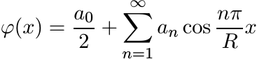
are nonnegative. Hence φ is positive definite.
5.2.16
Using 5.2.15 one can see that the following functions are positive definite:
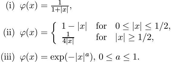
The special case a = 1 of (iii) was seen in 5.2.8. The next theorem provides a further extension.
5.2.17 Theorem
The function φ(x) = exp(−|x|a) is positive definite for 0 ≤ a ≤ 2.
Proof. Let 0 < a < 2. A calculation shows that
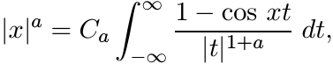
where
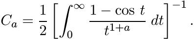
(The assumption a < 2 is needed to ensure that this last integral is convergent. At 0 the numerator in the integrand has a zero of order 2.) Thus we have
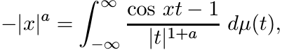
where dµ(t) = Ca dt. Let φn be defined as
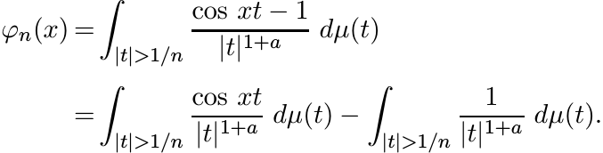
The second integral in the last line is a number, say cn, while the first is a function, say gn(x). This function is positive definite since cos xt is positive definite for all t. So, for each n, the function exp φn(x) is positive definite by Exercise 5.1.5 (iii). Since limn→∞ exp φn(x) = exp(−|x|a), this function too is positive definite for 0 < a < 2. Again, by continuity, this is true for a = 2 as well. ■
For a > 2 the function exp(−|x|a) is not positive definite. This is shown in Exercise 5.5.8.
5.2.18
The equality
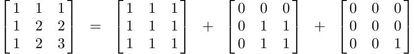
shows that the matrix on the left-hand side is positive. Thus the n × n matrix A with entries aij = min(i, j) is positive. This can be used to see that the kernel K(x, y) = min(x, y) is positive definite on [0, ∞) × [0, ∞).
5.2.19 Exercise
Let B be the n × n matrix with entries bij = 1/max(i, j). Show that this matrix is positive by an argument similar to the one in 5.2.18.
Note that if A is the matrix in 5.2.18, then B = DAD, where D = diag(1, 1/2, . . . , 1/n).
5.2.20 Exercise
Let λ1, . . . , λn be positive real numbers. Let A and B be the n × n matrices whose entries are aij = min(λi, λj) and bij = 1/ max(λi, λj), respectively. Show that A and B are positive definite.
5.2.21 Exercise
Show that the matrices A and B defined in Exercise 5.2.20 are infinitely divisible.
5.2.22 Exercise
Let 0 < λ1 ≤ λ2 ≤ · · · ≤ λn and let A be the symmetric matrix whose entries aij are defined as aij = λi/λj for 1 ≤ i ≤ j ≤ n. Show that A is infinitely divisible.
5.2.23 Exercise
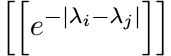
Let λ1, λ2, . . . , λn be real numbers. Show that the matrix A whose entries are
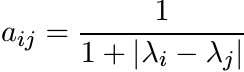
is infinitely divisible. [Hint: Use Pólya’s Theorem.]
5.3 LOEWNER MATRICES
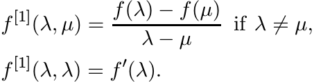
In this section we resume, and expand upon, our discussion of operator monotone functions. Recall some of the notions introduced at the end of Chapter 2. Let C1(I) be the space of continuously differentiable real-valued functions on an open interval I. The first divided difference of a function f in C1(I) is the function f[1] defined on I × I as
Let ![]() be the collection of all n × n Hermitian matrices whose eigenvalues are in I.
This is an open subset in the real vector space
be the collection of all n × n Hermitian matrices whose eigenvalues are in I.
This is an open subset in the real vector space ![]() consisting of all Hermitian matrices.
The function f induces a map from
consisting of all Hermitian matrices.
The function f induces a map from ![]() into
into ![]() .
.
If f ∈ C1(I) and ![]() we define f[1](A) as the matrix whose i, j entry is f[1](λi, λj),
where λ1, . . . , λn are the eigenvalues of A. This is called the Loewner matrix
of f at A.
we define f[1](A) as the matrix whose i, j entry is f[1](λi, λj),
where λ1, . . . , λn are the eigenvalues of A. This is called the Loewner matrix
of f at A.
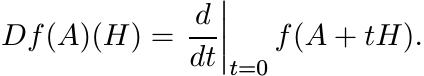
The function f on ![]() is differentiable. Its derivative at A, denoted as Df(A), is
a linear map on
is differentiable. Its derivative at A, denoted as Df(A), is
a linear map on ![]() characterized by the condition
characterized by the condition
for all ![]() . We have
. We have
 (5.19)
An interesting expression for this derivative in terms of Loewner matrices is given in the following theorem.
5.3.1 Theorem
Let f ∈ C1(I) and ![]() . Then
. Then
where ◦ denotes the Schur product in a basis in which A is diagonal.
One proof of this theorem can be found in MA (Theorem V.3.3). Here we give another proof based on different ideas.
Let [X, Y ] stand for the Lie bracket: [X, Y ] = XY − Y X. If X is Hermitian and Y skew-Hermitian, then [X, Y ] is Hermitian.
5.3.2 Theorem
Let f ∈ C1(I) and ![]() . Then for every skew-Hermitian matrix K
. Then for every skew-Hermitian matrix K
Proof. The exponential etK is a unitary matrix for all ![]() . From the series representation
of etK one can see that
. From the series representation
of etK one can see that
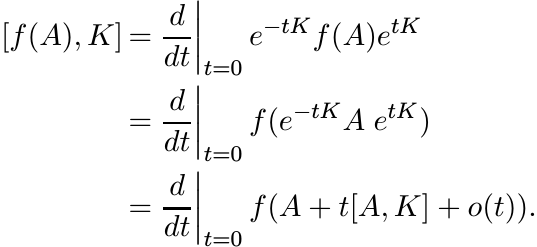
Since f is in the class C1, this is equal to
For each ![]() , the collection
, the collection
is a linear subspace of ![]() . On
. On ![]() we have an inner product
we have an inner product ![]() = tr XY . With respect to
this inner product, the orthogonal complement of CA is the space
= tr XY . With respect to
this inner product, the orthogonal complement of CA is the space
(It is easy to prove this. If H commutes with A, then
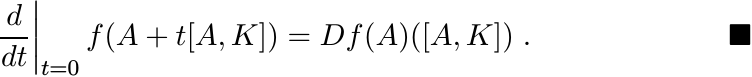
Proof of Theorem 5.3.1. Choose an orthonormal basis in which A = diag(λ1, . . . ,
λn). Let ![]() ; i.e., H = [A, K] for some skew-Hermitian matrix K. By (5.21), Df(A)(H)
= [f(A), K]. The entries of this matrix are
; i.e., H = [A, K] for some skew-Hermitian matrix K. By (5.21), Df(A)(H)
= [f(A), K]. The entries of this matrix are
These are the entries of f[1](A) ◦ H also. Thus the two sides of (5.20) are equal
when ![]() . Now let H belong to the complementary space
. Now let H belong to the complementary space ![]() . The theorem will be proved if
we show that the equality (5.20) holds in this case too. But this is easy. Since
H commutes with A, we may assume H too is diagonal, H = diag(h1, . . . , hn). In
this case the two sides of (5.20) are equal to the diagonal matrix with entries f′(λi)hi
on the diagonal. ■
. The theorem will be proved if
we show that the equality (5.20) holds in this case too. But this is easy. Since
H commutes with A, we may assume H too is diagonal, H = diag(h1, . . . , hn). In
this case the two sides of (5.20) are equal to the diagonal matrix with entries f′(λi)hi
on the diagonal. ■
The next theorem says that f is operator monotone on I if and only if for all n and
for all ![]() the Loewner matrices f[1](A) are positive. (This is a striking analogue
of the statement that a real function f is monotonically increasing if and only if
f′(t) ≥ 0.)
the Loewner matrices f[1](A) are positive. (This is a striking analogue
of the statement that a real function f is monotonically increasing if and only if
f′(t) ≥ 0.)
5.3.3 Theorem
Let f ∈ C1(I). Then f is operator monotone on I if and only if f[1](A) is positive for every Hermitian matrix A whose eigenvalues are contained in I.
Proof. Suppose f is operator monotone. Let ![]() and let H be the positive matrix with
all its entries equal to 1. For small positive t, A + tH is in
and let H be the positive matrix with
all its entries equal to 1. For small positive t, A + tH is in ![]() . We have A + tH ≥
A, and hence f(A + tH) ≥ f(A). This implies Df(A)(H) ≥ O. For this H, the right-hand
side of (5.20) is just f[1](A), and we have shown this is positive.
. We have A + tH ≥
A, and hence f(A + tH) ≥ f(A). This implies Df(A)(H) ≥ O. For this H, the right-hand
side of (5.20) is just f[1](A), and we have shown this is positive.
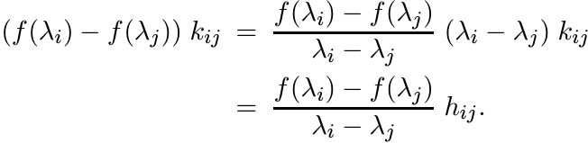
To prove the converse, let A0, A1 be matrices in ![]() with A1 ≥ A0. Let A(t) = (1 − t)A0
+ tA1, 0 ≤ t ≤ 1. Then A(t) is in
with A1 ≥ A0. Let A(t) = (1 − t)A0
+ tA1, 0 ≤ t ≤ 1. Then A(t) is in ![]() . Our hypothesis says that f[1](A(t)) is positive.
The derivative A′(t) = A1 − A0 is positive, and hence the Schur product f[1](A(t))
◦ A′(t) is positive. By Theorem 5.3.1 this product is equal to Df(A(t))(A′(t)). Since
. Our hypothesis says that f[1](A(t)) is positive.
The derivative A′(t) = A1 − A0 is positive, and hence the Schur product f[1](A(t))
◦ A′(t) is positive. By Theorem 5.3.1 this product is equal to Df(A(t))(A′(t)). Since
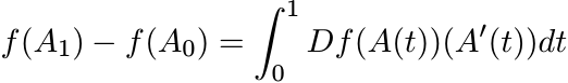
and the integrand is positive for all t, we have f(A1) ≥ f(A0). ■
We have seen some examples of operator monotone functions in Section 4.2. Theorem 5.3.3 provides a direct way of proving operator monotonicity of these and other functions. The positivity of the Loewner matrices f[1](A) is proved by associating with them some positive definite functions. Some examples follow.
5.3.4
The function
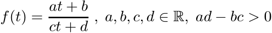
is operator monotone on any interval I that does not contain the point −d/c.
To see this write down the Loewner matrix f[1](A) for any A ∈ ![]() . If λ1, . . . , λn
are the eigenvalues of A, this Loewner matrix has entries
. If λ1, . . . , λn
are the eigenvalues of A, this Loewner matrix has entries
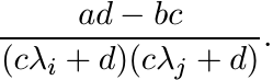
This matrix is congruent to the matrix with all entries 1, and is therefore positive.
5.3.5
The function f(t) = tr is operator monotone on (0, ∞) for 0 ≤ r ≤ 1.
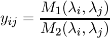
A Loewner matrix for this function is a matrix V with entries
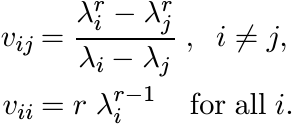
The numbers λi are positive and can, therefore, be written as exi for some xi. We have then
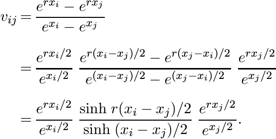
This matrix is congruent to the matrix with entries
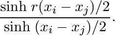
Since sinh rx/(sinh x) is a positive definite function for 0 ≤ r ≤ 1 (see 5.2.10), this matrix is positive.
5.3.6 Exercise
The function f(t) = tr is not operator monotone on (0, ∞) for any real number r outside [0, 1].
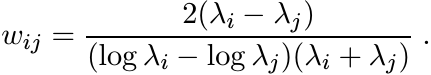
5.3.7
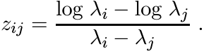
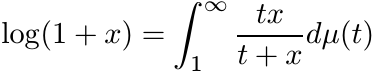
The function f(t) = log t is operator monotone on (0, ∞).
A Loewner matrix in this case has entries
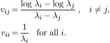
The substitution λi = exi reduces this to
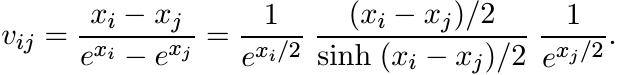
This matrix is positive since the function x/(sinh x) is positive definite. (See 5.2.9.)
Another proof of this is obtained from the equality
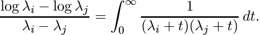
For each t the matrix [[1/(λi + t)(λj + t)]] is positive. (One more proof of operator monotonicity of the log function was given in Exercise 4.2.5.)
5.3.8
The function f(t) = tan t is operator monotone on ![]() .
.
In this case a Loewner matrix has entries
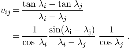
This matrix is positive since the function sin x/x is positive definite. (See 5.2.6.)
5.3.9 Exercise
For 0 ≤ r ≤ 1 let f be the map f(A) = Ar on the space of positive definite matrices. Show that
5.4 NORM INEQUALITIES FOR MEANS
The theme of this section is inequalities for norms of some expressions involving positive matrices. In the case of numbers they reduce to some of the most fundamental inequalities of analysis.
As a prototype consider the arithmetic-geometric mean inequality ![]() for positive numbers
a, b. There are many different directions in which one could look for a generalization
of this to positive matrices A, B. One version that involves the somewhat subtle
concept of a matrix geometric mean is given in Section 4.1. Instead of matrices we
could compare numbers associated with them. Thus, for example, we may ask whether
for positive numbers
a, b. There are many different directions in which one could look for a generalization
of this to positive matrices A, B. One version that involves the somewhat subtle
concept of a matrix geometric mean is given in Section 4.1. Instead of matrices we
could compare numbers associated with them. Thus, for example, we may ask whether
 (5.23)
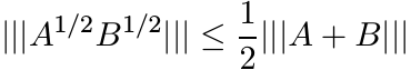
for every unitarily invariant norm. This is indeed true. There is a more general version of this inequality that is easier to prove: we have
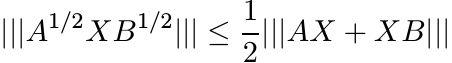 (5.24)
for every X. What makes it easier is a lovely trick. It is enough to prove (5.24) in the special case A = B. (The inequality (5.23) is a vacuous statement in this case.) Suppose we have proved
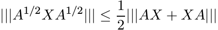 (5.25)
for all matrices X and positive A. Then given X and positive A, B we may replace
A and X in (5.25) by the 2 × 2 block matrices ![]() and
and ![]() . This gives the inequality (5.24).
. This gives the inequality (5.24).
Since the norms involved are unitarily invariant we may assume that A is diagonal, A = diag(λ1, . . . , λn). Then we have
 (5.26)
where Y is the matrix with entries
 (5.27)
This matrix is congruent to the Cauchy matrix—the one whose entries are 1/(λi + λj). Since that matrix is positive (Exercise 1.1.2) so is Y . All the diagonal entries of Y are equal to 1. So, using Exercise 2.7.12 we get the inequality (5.25) from (5.26).
The inequalities that follow are proved using similar arguments. Matrices that occur in the place of (5.27) are more complicated and their positivity is not as easy to establish. But in Section 5.2 we have done most of the work that is needed.
5.4.1 Theorem
Let A, B be positive and let X be any matrix. Then for 0 ≤ ν ≤ 1 we have
Proof. Follow the arguments used above in proving (5.24). To prove the second inequality in (5.28) we need to prove that the matrix Y whose entries are
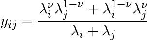 (5.29)
is positive for 0 < ν < 1. (When ν = 1/2 this reduces to (5.27).) Writing
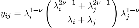
we see that Y is congruent to the matrix Z whose entries are
This matrix is like the one in 5.3.5. The argument used there reduces the question of positivity of Z to that of positive definiteness of the function cosh αx/(cosh x) for −1 < α < 1. In 5.2.10 we have seen that this function is indeed positive definite. The proof of the first inequality in (5.28) is very similar to this, and is left to the reader. ■
5.4.2 Exercise
Show that for 0 ≤ ν ≤ 1
5.4.3 Exercise
For the Hilbert-Schmidt norm we have
for positive matrices A and 0 < ν < 1. This is not always true for the operator norm || · ||.
5.4.4 Exercise
For any matrix Z let
Let A be a positive matrix and let X be a Hermitian matrix. Let S = AνXA1−ν, T = νAX + (1 − ν)XA. Show that for 0 ≤ ν ≤ 1
In Chapter 4 we defined the logarithmic mean of a and b. This is the quantity
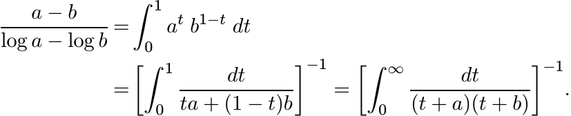 (5.32)
A proof of the inequality (4.3) using the ideas of Section 5.3 is given below.
5.4.5 Lemma
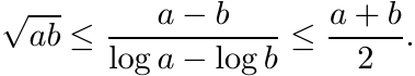 (5.33)
Proof. Put a = ex and b = ey. A small calculation reduces the job of proving the first inequality in (5.33) to showing that t ≤ sinh t for t > 0, and the second to showing that tanh t ≤ t for all t > 0. Both these inequalities can be proved very easily. ■
5.4.6 Exercise
Show that for A, B positive and for every X
 (5.34)
This matrix version of the arithmetic-logarithmic-geometric mean inequality can be generalized to all unitarily invariant norms.
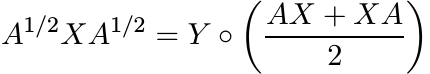
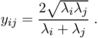
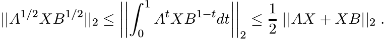
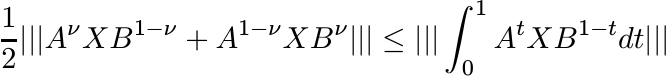
5.4.7 Theorem
For every unitarily invariant norm we have
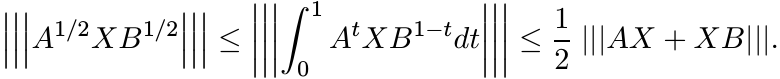 (5.35)
Proof. The idea of the proof is very similar to that of Theorem 5.4.1. Assume B =
A, and suppose A is diagonal with entries λ1, . . . , λn on the diagonal. The matrix
A1/2XA1/2 is obtained from ![]() by entrywise multiplication with the matrix Y whose entries
are
by entrywise multiplication with the matrix Y whose entries
are
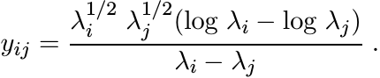
This matrix is congruent to one with entries
We have seen in 5.3.7 that this matrix is positive. That proves the first inequality in (5.35).
The matrix ![]() is the Schur product of
is the Schur product of ![]() with the matrix W whose entries are
with the matrix W whose entries are
Making the substitution λi = exi, we have
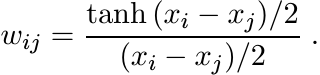
This matrix is positive since the function tanh x/x is positive definite. (See 5.2.11.) That proves the second inequality in (5.35). ■
5.4.8 Exercise
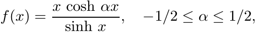
A refinement of the inequalities (5.28) and (5.35) is provided by the assertion
for 1/4 ≤ ν ≤ 3/4. Prove this using the fact that (x cosh αx)/ sinh x is a positive definite function for −1/2 ≤ α ≤ 1/2. (See 5.2.10.)
5.4.9 Exercise
Let H, K be Hermitian, and let X be any matrix. Show that
This is a matrix version of the inequality |sin x| ≤ |x|.
5.4.10 Exercise
Let H, K and X be as above. Show that
5.4.11 Exercise
Let A, B be positive matrices. Show that
Hence, if H, K are Hermitian, then
for every matrix X.
5.5 THEOREMS OF HERGLOTZ AND BOCHNER
These two theorems give complete characterizations of positive definite sequences and positive definite functions, respectively. They have important applications throughout analysis. For the sake of completeness we include proofs of these theorems here. Some basic facts from functional analysis and Fourier analysis are needed for the proofs. The reader is briefly reminded of these facts.
Let M[0, 1] be the space of complex finite Borel measures on the interval [0, 1].
This is equipped with a norm ![]() , and is the Banach space dual of the space C[0, 1].
If
, and is the Banach space dual of the space C[0, 1].
If ![]() converges to
converges to ![]() for every f ∈ C[0, 1], we say that the sequence {µn} in M[0, 1]
converges to µ in the weak∗ topology.
for every f ∈ C[0, 1], we say that the sequence {µn} in M[0, 1]
converges to µ in the weak∗ topology.
A basic fact about this convergence is the following theorem called Helly’s Selection Principle.
5.5.1 Theorem
Let {µn} be a sequence of probability measures on [0, 1]. Then there exists a probability measure µ and a subsequence {µm} of {µn} such that µm converges in the weak∗ topology to µ.
Proof. The space C[0, 1] is a separable Banach space. Choose a sequence {fj} in C[0,
1] that includes the function 1 and whose linear combinations are dense in C[0, 1].
Since ||µn|| = 1, for each j we have ![]() for all n. Thus for each j
for all n. Thus for each j![]() is a bounded sequence
of positive numbers. By the diagonal procedure, we can extract a subsequence {µm}
such that for each j, the sequence
is a bounded sequence
of positive numbers. By the diagonal procedure, we can extract a subsequence {µm}
such that for each j, the sequence ![]() converges to a limit, say ξj, as m → ∞.
converges to a limit, say ξj, as m → ∞.
If ![]() is any (finite) linear combination of the fj, let
is any (finite) linear combination of the fj, let
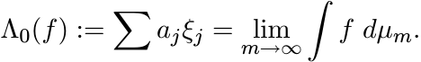
This is a linear functional on the linear span of {fj}, and |Λ0(f)| ≤ ||f|| for every
f in this span. By continuity Λ0 has an extension Λ to C[0, 1] that satisfies |Λ(f)|
≤ ||f|| for all f in C[0, 1]. This linear functional Λ is positive and unital. So,
by the Riesz Representation Theorem, there exists a probability measure µ on [0,
1] such that ![]() for all f ∈ C[0, 1].
for all f ∈ C[0, 1].
Finally, we know that ![]() converges to
converges to ![]() for every f in the span of {fj}. Since such
f are dense and the µm are uniformly bounded, this convergence persists for every
f in C[0, 1]. ■
for every f in the span of {fj}. Since such
f are dense and the µm are uniformly bounded, this convergence persists for every
f in C[0, 1]. ■
Theorem 5.5.1 is also a corollary of the Banach Alaoglu theorem. This says that the closed unit ball in the dual space of a Banach space is compact in the weak∗ topology. If a Banach space X is separable, then the weak∗ topology on the closed unit ball of its dual X∗ is metrizable.
5.5.2 Herglotz’ Theorem
Let ![]() be a positive definite sequence and suppose a0 = 1. Then there exists a probability
measure µ on [−π, π] such that
be a positive definite sequence and suppose a0 = 1. Then there exists a probability
measure µ on [−π, π] such that
 (5.36)
Proof. The positive definiteness of {an} implies that for every real x we have
This inequality can be expressed in another form
Let fN(x) be the function given by the last sum. Then
For any Borel set E in [−π, π], let
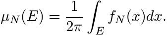
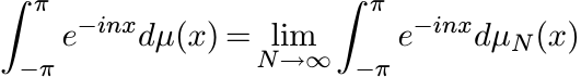
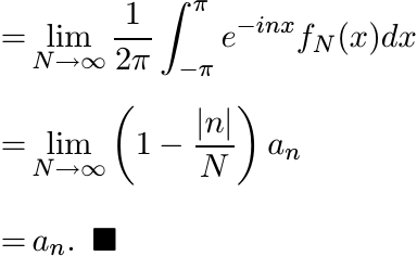
Then µN is a probability measure on [−π, π]. Apply Helly’s selection principle to the sequence {µN }. There exists a probability measure µ to which (a subsequence of ) µN converges in the weak∗ topology. Thus for every n
We remark that the sum
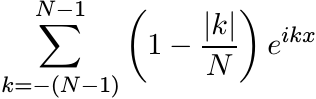
is called the Fejér kernel and is much used in the study of Fourier series.
The condition a0 = 1 in the statement of Herglotz’ theorem is an inessential normalization. This can be dropped; then µ is a finite positive measure with ||µ|| = a0.
Bochner’s theorem, in the same spirit as Herglotz’, says that every continuous positive
definite function on ![]() is the Fourier-Stieltjes transform of a finite positive measure
on R. The proof needs some approximation arguments. For the convenience of the reader
let us recall some basic facts.
is the Fourier-Stieltjes transform of a finite positive measure
on R. The proof needs some approximation arguments. For the convenience of the reader
let us recall some basic facts.
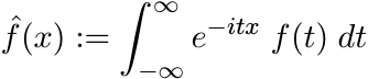
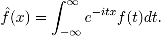
For ![]() we write
we write ![]() for its Fourier transform defined as
for its Fourier transform defined as
This function is in ![]() , the class of continuous functions vanishing at ∞. We write
, the class of continuous functions vanishing at ∞. We write
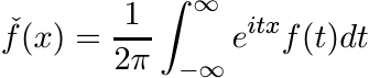
for the inverse Fourier transform of f. If the function ![]() is in
is in ![]() (and this is not
always the case) then
(and this is not
always the case) then ![]()
The Fourier transform on the space ![]() is defined as follows. Let
is defined as follows. Let ![]() . Then
. Then ![]() is defined
as above. One can see that
is defined
as above. One can see that ![]() and the map
and the map ![]() is an L2-isometry on the space
is an L2-isometry on the space ![]() . This space
is dense in
. This space
is dense in ![]() . So the isometry defined on it has a unique extension to all of
. So the isometry defined on it has a unique extension to all of ![]() . This
unitary operator on
. This
unitary operator on ![]() is denoted again by
is denoted again by ![]() . The inverse of the map
. The inverse of the map ![]() is defined by
inverting this unitary operator. The fact that the Fourier transform is a bijective
map of
is defined by
inverting this unitary operator. The fact that the Fourier transform is a bijective
map of ![]() onto itself makes some operations in this space simpler.
onto itself makes some operations in this space simpler.
Let δR be the function defined in 5.2.14. The family {δN} is an approximate identity: as N → ∞, the convolution δN ∗ g converges to g in an appropriate sense. The “appropriate sense” for us is the following.
If g is either an element of ![]() , or a bounded measurable function, then
, or a bounded measurable function, then
 (5.37)
In the discussion that follows we ignore constant factors involving 2π. These do not affect our conclusions in any way.
The Fourier transform “converts convolution into multiplication;” i.e.,
The Riesz representation theorem and Helly’s selection principle have generalizations
to the real line. The space ![]() is a separable Banach space. Its dual is the space
is a separable Banach space. Its dual is the space ![]() of finite Borel measures on
of finite Borel measures on ![]() with norm
with norm ![]() . Every bounded sequence {µn} in
. Every bounded sequence {µn} in ![]() has a weak∗
convergent subsequence {µm}; i.e., for every
has a weak∗
convergent subsequence {µm}; i.e., for every ![]() converges to
converges to ![]() . This too is a special
case of the Banach-Alaoglu theorem.
. This too is a special
case of the Banach-Alaoglu theorem.
5.5.3 Bochner’s Theorem
Let φ be any function on the real line that is positive definite and continuous at 0. Then there exists a finite positive measure µ such that
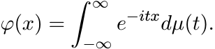 (5.38)
Proof. By Lemma 5.1.2, φ is continuous everywhere. Suppose in addition that ![]() . Using
(5.6) we see that
. Using
(5.6) we see that
 (0)
(0)
Thus φ is in the space ![]() also. Hence, there exists
also. Hence, there exists ![]() such that
such that
 (5.39)
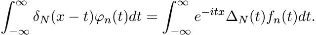
Let ∆N(x) be the tent function defined in (5.16). Then
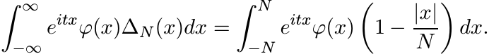 (5.40)
This integral (of a continuous function over a bounded interval) is a limit of Riemann sums. Let xj = j N/K, −K ≤ j ≤ K. The last integral is the limit, as K → ∞, of sums
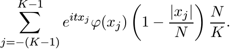
These sums can be expressed in another way:
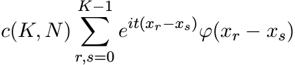 (5.41)
where c(K, N) is a positive number. (See the proof of Herglotz’ theorem where two sums of this type were involved.) Since φ is positive definite, the sum in (5.41) is nonnegative. Hence, the integral (5.41), being the limit of such sums, is nonnegative. As N → ∞ the integral in (5.40) tends to the one in (5.39). So, that integral is nonnegative too. Thus f(t) ≥ 0.
Now let φ be any continuous positive definite function and let
Since φ is bounded, φn is integrable. Since φ(x) and e−x2/n are positive definite, so is their product φn(x). Thus by what we have proved in the preceding paragraph, for each n
We have the relation δN ∗ φn = (∆Nfn)^, i.e.,
 (5.42)
At x = 0 this gives
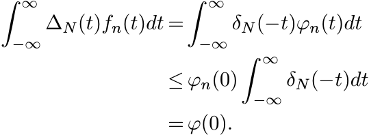
Let N → ∞. This shows
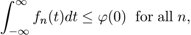 (0)
(0)
i.e., ![]() and ||fn||1 ≤ φ(0). Let dµn(t) = fn(t)dt. Then {µn} are positive measures
on
and ||fn||1 ≤ φ(0). Let dµn(t) = fn(t)dt. Then {µn} are positive measures
on ![]() and ||µn|| ≤ φ(0). So, by Helly’s selection principle, there exists a positive
measure µ, with ||µ|| ≤ φ(0), to which (a subsequence of ) µn converges in the weak∗
topology.
and ||µn|| ≤ φ(0). So, by Helly’s selection principle, there exists a positive
measure µ, with ||µ|| ≤ φ(0), to which (a subsequence of ) µn converges in the weak∗
topology.
The equation (5.42) says
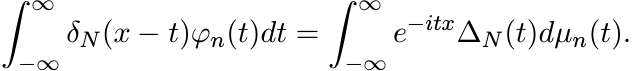 (5.43)
Keep N fixed and let n → ∞. For the right-hand side of (5.43) use the weak∗ convergence of µn to µ, and for the left-hand side the Lebesgue-dominated convergence theorem. This gives
 (5.44)
Now let N → ∞. Since φ is a bounded measurable function, by (5.37) the left-hand side of (5.44) goes to φ(x) a.e. The right-hand side converges by the bounded convergence theorem. This shows
Since the two sides are continuous functions of x, this equality holds everywhere. ■
Of the several examples of positive definite functions in Section 5.2 some were shown to be Fourier transforms of nonnegative integrable functions. (See 5.2.5 - 5.2.8.) One can do this for some of the other functions too.
5.5.4
The list below gives some functions φ and their Fourier transforms φ![]() (ignoring constant
factors).
(ignoring constant
factors).
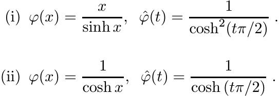
Let φ be a continuous positive definite function. Then the measure µ associated with φ via the formula (5.38) is a probability measure if and only if φ(0) = 1. In this case φ is called a characteristic function.
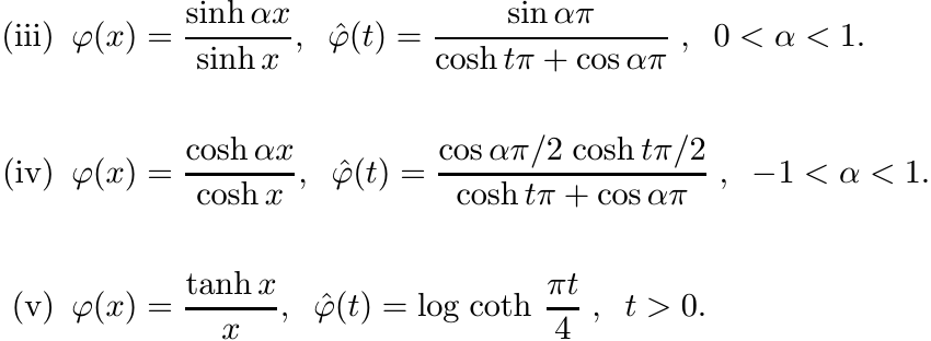
5.5.5 Proposition
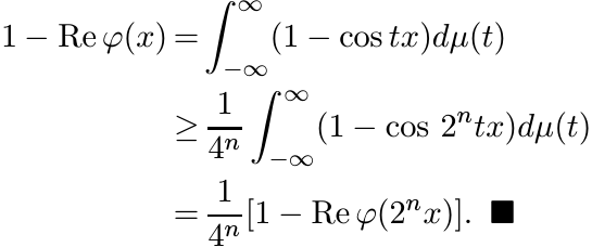
Let φ be a characteristic function. Then
for all x and n = 1, 2, . . . .
Proof. By elementary trigonometry

An iteration leads to the inequality
From (5.38) we have
5.5.6 Corollary
Suppose φ is a positive definite function and φ(x) = φ(0) + o(x2); i.e.,
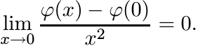 (0)
(0)Then φ is a constant.
Proof. We may assume that φ(0) = 1. Then using the Proposition above we have for all x and n

The hypothesis on φ implies that the last expression goes to zero as n → ∞. Hence, Re φ(x) = 1 for all x. But then φ(x) ≡ 1. ■
5.5.7 Exercise
Suppose φ is a characteristic function, and φ(x) = 1 + o(x) + o(x2) in a neighbourhood of 0, where o(x) is an odd function. Then φ ≡ 1. [Hint: consider φ(x)φ(−x).]
5.5.8 Exercise
The functions e−x4 , 1/(1 + x4), and e−|x|a for a > 2, are not positive definite.
Bochner’s theorem can be used also to show that a certain function is not positive definite by showing that its Fourier transform is not everywhere nonnegative.
5.5.9 Exercise
Use the method of residues to show that for all t > 0
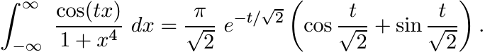
It follows from Bochner’s theorem that the function f(x) = 1/(1 + x4) is not positive definite.
5.6 SUPPLEMENTARY RESULTS AND EXERCISES
5.6.1 Exercise
Let U be a unitary operator on any separable Hilbert space ![]() . Show that for each unit
vector x in
. Show that for each unit
vector x in ![]() the sequence
the sequence
is positive definite.
This observation is the first step on one of the several routes to the spectral theorem for operators in Hilbert space. We indicate this briefly.
Let U be a unitary operator on ![]() . By Exercise 5.6.1 and Herglotz’ theorem, for each
unit vector x in
. By Exercise 5.6.1 and Herglotz’ theorem, for each
unit vector x in ![]() , there exists a probability measure µx on the interval [−π, π]
such that
, there exists a probability measure µx on the interval [−π, π]
such that
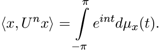 (5.46)
Using a standard technique called polarisation, one can obtain from this, for each pair x, y of unit vectors a complex measure µx,y such that
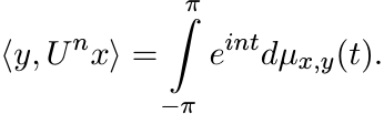 (5.47)
Now for each Borel subset E ⊂ [−π, π] let P(E) be the operator on ![]() defined by the
relation
defined by the
relation
It can be seen that P(E) is an orthogonal projection and that P(·) is countably additive on the Borel σ-algebra of [−π, π]. In other words P(·) is a projection-valued measure. We can then express U as an integral
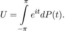 (5.49)
This is the spectral theorem for unitary operators. The spectral theorem for self-adjoint operators can be obtained from this using the Cayley transform.
5.6.2 Exercise
Let B be an n × n Hermitian matrix. Show that for each unit vector u the function
is a positive definite function on ![]() . Use this to show that the functions tr eitB
and det eitB are positive definite.
. Use this to show that the functions tr eitB
and det eitB are positive definite.
5.6.3 Exercise
Let A, B be n × n Hermitian matrices and let
Is φ a positive definite function? Show that this is so if A and B commute.
The general case of the question raised above is a long-standing open problem in quantum statistical mechanics. The Bessis-Moussa-Villani conjecture says that the function φ in (5.50) is positive definite for all Hermitian matrices A and B.
The purpose of the next three exercises is to calculate Fourier transforms of some functions that arose in our discussion.
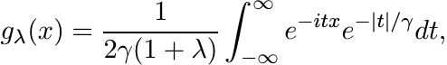
5.6.4 Exercise
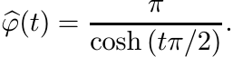
Let φ(x) = 1/cosh x. Its Fourier transform is
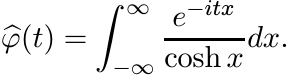
This integral may be evaluated by the method of residues. Let f be the function
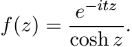
Then
For any R > 0 the rectangular contour with vertices −R, R, R+iπ and −R + iπ contains one simple pole, z = iπ/2, of f inside it. Integrate f along this contour and then let |R| → ∞. The contribution of the two vertical sides goes to zero. So
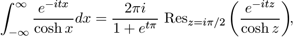
where Resz=z0 f(z) is the residue of f at a pole z0.
A calculation shows that
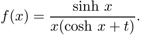
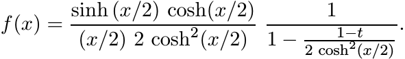
5.6.5 Exercise
More generally consider the function
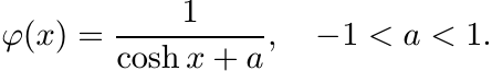 (5.51)
Integrate the function
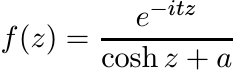
along the rectangular contour with vertices −R, R, R + i2π and −R + i2π. The function f has two simple poles z = i(π ± arccos a) inside this rectangle. Proceed as in Exercise 5.6.4 to show
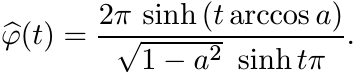 (5.52)
It is plain that ![]() . Hence by Bochner’s theorem φ(x) is positive definite for −1 <
a < 1. By a continuity argument it is positive definite for a = 1 as well.
. Hence by Bochner’s theorem φ(x) is positive definite for −1 <
a < 1. By a continuity argument it is positive definite for a = 1 as well.
5.6.6 Exercise
Now consider the function
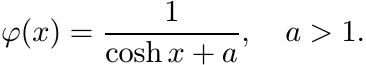 (5.53)
Use the function f and the rectangular contour of Exercise 5.6.5. Now f has two simple poles z = ± arccosh t+iπ inside this rectangle. Show that
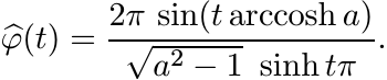 (5.54)
It is plain that ![]() is negative for some values of t. So the function φ in (5.53) is
not positive definite for any a > 1.
is negative for some values of t. So the function φ in (5.53) is
not positive definite for any a > 1.
5.6.7 Exercise
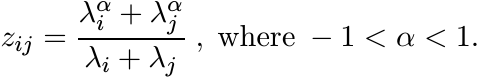
Let λ1, . . . , λn be positive numbers and let Z be the n× n matrix with entries
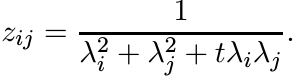
Show that if −2 < t ≤ 2, then Z is positive definite; and if t > 2 then there exists an n > 2 for which this matrix is not positive definite. (See Exercise 1.6.4.)
5.6.8 Exercise
For 0 < a < 1, let fa be the piecewise linear function defined as
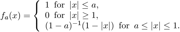
Show that fa is not positive definite. Compare this with 5.2.13 and 5.2.15. Express fa as the convolution of two characteristic functions.
The technique introduced in Section 4 is a source of several interesting inequalities. The next two exercises illustrate this further.
5.6.9 Exercise
(i) Let A be a Hermitian matrix. Use the positive definiteness of the function sech x to show that for every matrix X
(ii)
Now let A be any matrix. Apply the result of (i) to the matrices ![]() and show that
and show that
for every matrix X. Replacing A by iA, one gets
5.6.10 Exercise
Let A, B be normal matrices with ||A|| ≤ 1 and ||B|| ≤ 1. Show that for every X we have
The inequalities proved in Section 5.4 have a leitmotiv. Let M(a, b) be any mean of positive numbers a and b satisfying the conditions laid down at the beginning of Chapter 4. Let A be a positive definite matrix with eigenvalues λ1 ≥ · · · ≥ λn. Let M(A, A) be the matrix with entries
Many of the inequalites in Section 5.4 say that for certain means M1 and M2
for all X. We have proved such inequalites by showing that the matrix Y with entries
 (5.56)
is positive definite. This condition is also necessary for (5.55) to be true for all X.
5.6.11 Proposition
Let M1(a, b) and M2(a, b) be two means. Then the inequality (5.55) is true for all X if and only if the matrix Y defined by (5.56) is positive definite.
Proof. The Schur product by Y is a linear map on ![]() . The inequality (5.55) says that
this linear map on the space
. The inequality (5.55) says that
this linear map on the space ![]() equipped with the norm || · || is contractive. Hence
it is contractive also with respect to the dual norm || · ||1; i.e.,
equipped with the norm || · || is contractive. Hence
it is contractive also with respect to the dual norm || · ||1; i.e.,
Choose X to be the matrix with all entries equal to 1. This gives ||Y ||1 ≤ n. Since Y is Hermitian
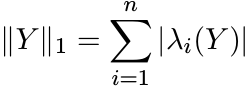
where λi(Y ) are the eigenvalues of Y. Since yii = 1 for all i, we have
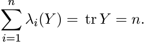
Thus ![]() . But this is possible only if λi(Y ) ≥ 0 for all i. In other words Y is positive.
■
. But this is possible only if λi(Y ) ≥ 0 for all i. In other words Y is positive.
■
Let us say that M1 ≤ M2 if M1(a, b) ≤ M2(a, b) for all positive numbers a and b; and M1 << M2 if for every n and every choice of n positive numbers λ1, . . . , λn the matrix (5.56) is positive definite. If M1 << M2 the inequality (5.55) is true for all positive matrices A and all matrices X. Clearly M1 ≤ M2 if M1 << M2. The converse is not always true.
5.6.12 Exercise
Let A(a, b) and G(a, b) be the arithmetic and the geometric means of a and b. For 0 ≤ α ≤ 1 let
Clearly we have Fα ≤ Fβ whenever α ≤ β. Use Exercise 5.6.6 to show that Fα <<
Fβ if and only if ![]() .
.
Using Exercise 2.7.12 one can see that if M1 << M2, then the inequality (5.55) is true for all unitarily invariant norms. The weaker condition M1 ≤ M2 gives this inequality only for the Hilbert-Schmidt norm || · ||2.
In Exercises 1.6.3, 1.6.4, 5.2.21, 5.2.22 and 5.2.23 we have outlined simple proofs of the infinite divisibility of some special matrices. These proofs rely on arguments specifically tailored to suit the matrices at hand. In the next few exercises we sketch proofs of some general theorems that are useful in this context.
An n × n Hermitian matrix A is said to be conditionally positive definite if ![]() for
all
for
all ![]() such that x1 + · · · + xn = 0. (The term almost positive definite is also used
sometimes.)
such that x1 + · · · + xn = 0. (The term almost positive definite is also used
sometimes.)
5.6.13 Proposition
Let A = [[aij]] be an n × n conditionally positive definite matrix. Then there exist
a positive definite matrix B = [[bij]] and a vector y = (y1, . . . , yn) in ![]() such
that
such
that
Proof. Let J be the n × n matrix all of whose entries are equal to 1/n. For any vector
![]() let x# = Jx and
let x# = Jx and ![]() . Since
. Since ![]() we have
we have
Let B = A − AJ − JA + JAJ. The inequality above says that
In other words B is positive definite.
If C1, . . . , Cn are the columns of the matrix A, then the jth column of the matrix
JA has all its entries equal to ![]() , the number obtained by averaging the entries of
the column Cj. Likewise, if R1, . . . , Rn are the rows of A, then the ith row of
AJ has all its entries equal to
, the number obtained by averaging the entries of
the column Cj. Likewise, if R1, . . . , Rn are the rows of A, then the ith row of
AJ has all its entries equal to ![]() . Since A is Hermitian
. Since A is Hermitian ![]() is the complex conjugate
of
is the complex conjugate
of ![]() . The matrix JAJ has all its entries equal to
. The matrix JAJ has all its entries equal to ![]() . Thus the i, j entry of the matrix
AJ + JA − JAJ is equal to
. Thus the i, j entry of the matrix
AJ + JA − JAJ is equal to ![]() . Let y be the vector
. Let y be the vector
 (5.57)
Then the equation (5.57) is satisfied. ■
5.6.14 Exercise
Let A = [[aij]] be a conditionally positive definite matrix. Show that the matrix [[eaij ]] is positive definite. [Hint: If B = [[bij]] is positive definite, then [[ebij ]] is positive definite. Use Proposition 5.6.13.]
5.6.15 Exercise
Let A = [[aij]] be an n × n matrix with positive entries and let L = [[log aij]]. Let E be the matrix all whose entries are equal to 1. Note that Ex = 0 if x1 + · · · + xn = 0.
(i) Suppose A is infinitely divisible. Let x be any vector with x1 + · · · + xn = 0, and for r > 0 let A(r) be the matrix with entries arij. Then
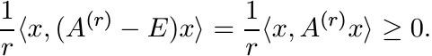
Let r ↓ 0. This gives
Thus L is conditionally positive definite.
(ii) Conversely, if L is conditionally positive definite, then so is rL for every r ≥ 0. Use Exercise 5.6.14 to show that this implies A is infinitely divisible.
Thus a Hermitian matrix A with entries aij > 0 is infinitely divisible if and only if the matrix L = [[log aij]] is conditionally positive definite. The next exercise gives a criterion for conditional positive definiteness.
5.6.16 Exercise
Given an n×n Hermitian matrix B = [[bij]] let D be the (n−1)×(n−1) matrix with entries
Show that B is conditionally positive definite if and only if D is positive definite.
We now show how the results of Exercises 5.6.14–5.6.16 may be used to prove the infinite divisibility of an interesting matrix.
For any n, the n × n Pascal matrix A is the matrix with entries
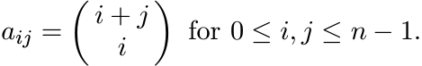 (5.59)
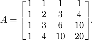
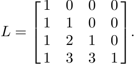
The entries of the Pascal triangle occupy the antidiagonals of A. Thus the 4 × 4 Pascal matrix is
5.6.17 Exercise
Prove the combinatorial identity
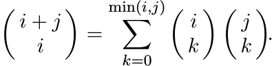
[Hint: Separate i + j objects into two groups, the first containing i objects and the second j objects. If we choose i − k objects from the first group and k from the second, we have chosen i objects out of i + j.]
5.6.18 Exercise
Show that
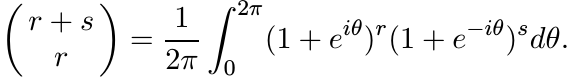
Use this to conclude that the Pascal matrix is a Gram matrix and is thus positive definite.
5.6.19 Exercise
Let L be the n × n lower triangular matrix whose rows are the rows of the Pascal triangle. Thus for n = 4
Show that A = LL∗. This gives another proof of the positive definiteness of the Pascal matrix A.
5.6.20 Exercise
For every n, the n × n Pascal matrix is infinitely divisible. Prove this statement following the steps given below.
(i) Use the results of Exercises 5.6.15 and 5.6.16. If B has entries bij = log aij, where aij are defined by (5.59), then the entries dij defined by (5.58) are given by
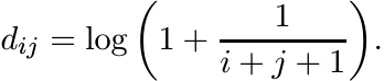
We have to show that the matrix D = [[dij]] is positive definite.
(ii) For x > 0 we have
where µ is the probability measure on [0, ∞) defined as dµ(t) = dt/t2. Use this to show that
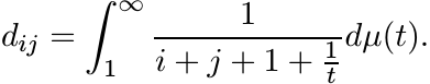
(iii) Thus the matrix D can be expressed as
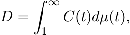
where C(t) = [[cij(t)]] is a Cauchy matrix for all t ≥ 1. This shows that D is positive definite.
5.6.21 Exercise
The infinite divisibility of the Pascal matrix can be proved in another way as follows. Let λ1, . . . , λn be positive numbers, and let K be the n × n matrix with entries
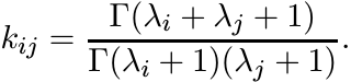
When λj = j, 1 ≤ j ≤ n, this is the Pascal matrix. Use Gauss’s product formula for the gamma function
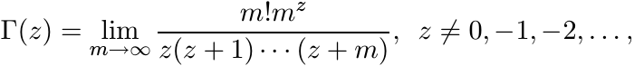
to see that
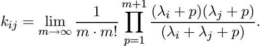
Each of the factors in this product is the i, j entry of a matrix that is congruent to a Cauchy matrix. Hence K is infinitely divisible.
Let f be a nonnegative function on ![]() . If for each r > 0 the function (f(x))r is
positive definite, then we say that f is an infinitely divisible function. By Schur’s
theorem, the product of two infinitely divisible functions is infinitely divisible.
If f is a nonnegative function and for each m = 1, 2, . . . the function (f(x))1/m
is positive definite, then f is infinitely divisible.
. If for each r > 0 the function (f(x))r is
positive definite, then we say that f is an infinitely divisible function. By Schur’s
theorem, the product of two infinitely divisible functions is infinitely divisible.
If f is a nonnegative function and for each m = 1, 2, . . . the function (f(x))1/m
is positive definite, then f is infinitely divisible.
Some examples of infinitely divisible functions are given in the next few exercises.
5.6.22 Exercise
(i) The function f(x) = 1/(cosh x) is infinitely divisible.
(ii) The function f(x) = 1/(cosh x + a) is infinitely divisible for −1 < a ≤ 1. [Hint: Use Exercises 1.6.4 and 1.6.5.]
5.6.23 Exercise
In Section 5.2.10 we saw that the function
is positive definite. Using this information and Schur’s theorem one can prove that f is in fact infinitely divisible. The steps of the argument are outlined.
(i)
Let a and b be any two nonnegative real numbers. Then either ![]() is positive definite.
is positive definite.
Hence
is positive definite.
(ii) Use the identity
to obtain
(iii) For 0 < r < 1 we have the expansion
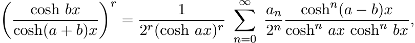
where the coefficients an are nonnegative. Use Part (i) of this exercise and of Exercise 5.6.22 to prove that the series above represents a positive definite function. This establishes the assertion that (cosh αx)/(cosh x) is infinitely divisible for 0 < α < 1.
5.6.24 Exercise
The aim of this exercise is to show that the function
is infinitely divisible. Its positive definiteness has been established in Section 5.2.10.
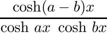
(i) Imitate the arguments in Exercise 5.6.23. Use the identity
to show that the function
is infinitely divisible for 0 ≤ b ≤ a. (This restriction is needed to handle the term sinh(a − b)x occurring in the series expansion.) This shows that the function (sinh αx)/(sinh x) is infinitely divisible for 1/2 ≤ α ≤ 1.
(ii) Let α be any number in (0, 1) and choose a sequence
where αi/αi+1 ≥ 1/2. Then
Each factor in this product is infinitely divisible, and hence so is the product.
5.6.25 Exercise
(i) Use Exercise 5.6.24 to show that the function x/(sinh x) is infinitely divisible. [Hint: Take limit α ↓ 0.]
(ii) Use this and the result of Exercise 5.6.23 to show that the function
is infinitely divisible.
5.6.26 Exercise
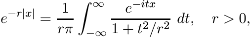
Let λ1, . . . , λn be any real numbers. Use the result of Exercise 5.2.22 to show that the matrix
is infinitely divisible. Thus the function f(x) = e−|x| is infinitely divisible. Use the integral formula
to obtain another proof of this fact.
5.6.27 Exercise
Using the gamma function, as in Exercise 1.6.4, show that for every r > 0
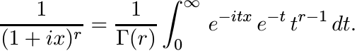
Thus the functions 1/(1 + ix)r, 1/(1 − ix)r, and 1/(1 + x2)r are positive definite for every r > 0. This shows that 1/(1 + x2) is infinitely divisible.
5.6.28 Exercise
Let a and b be nonnegative numbers with a ≥ b. Let 0 < r < 1. Use the integral formula (1.39) to show that
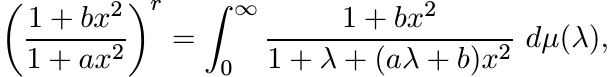
where µ is a positive measure. This is equal to
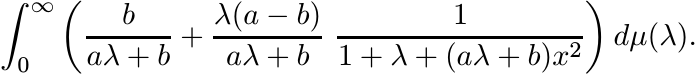
Show that this is positive definite as a function of x. Note that it suffices to show that for each λ > 0,
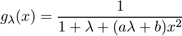
is positive definite. This, in turn, follows from the integral representation
where γ = [(aλ + b)/(1 + λ)]1/2. Thus, for a ≥ b the function f(x) = (1 + bx2)/(1 + ax2) is infinitely divisible.
5.6.29 Exercise
Show that the function f(x) = (tanh x)/x is infinitely divisible. [Hint: Use the infinite product expansion for f(x).]
5.6.30 Exercise
Let t > −1 and consider the function
Use the identity
to obtain the equality
Use the binomial theorem and Exercise 5.6.29 to prove that f is infinitely divisible for −1 < t ≤ 1.
Thus many of the positive definite functions from Section 5.2 are infinitely divisible. Consequently the associated positive definite matrices are infinitely divisible. In particular, for any positive numbers λ1, . . . , λn the n × n matrices V, W and Y whose entries are, respectively,
are infinitely divisible.
5.6.31 Another proof of Bochner’s Theorem
The reader who has worked her way through the theory of Pick functions (as given in Chapter V of MA) may enjoy the proof outlined below.
(i)
Let φ be a positive definite function on ![]() , continuous at 0. Let z = x + iy be a complex
number and put
, continuous at 0. Let z = x + iy be a complex
number and put
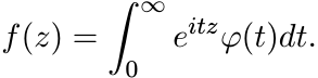 (5.60)
Since φ is bounded, this integral is convergent for y > 0. Thus f is an analytic function on the open upper half-plane H+.
(ii) Observe that
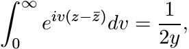
and so from (5.60) we have
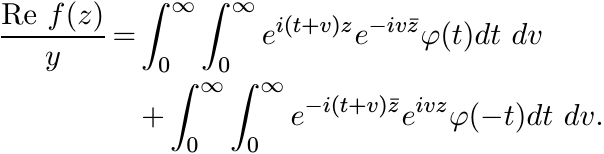
First substitute u = t + v in both the integrals, and then interchange u and v in the second integral to obtain
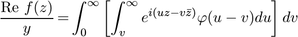
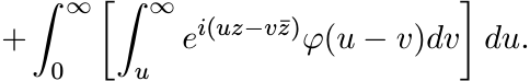
Observe that these two double integrals are over the quarter-planes {(u, v) : u ≥ v ≥ 0} and {(u, v) : v ≥ u ≥ 0}, respectively. Hence
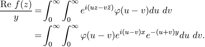
Since φ is a positive definite function, this integral is nonnegative. (Write it as a limit of Riemann sums each of which is nonnegative.)
Thus f maps the upper half-plane into the right half-plane. So i f(z) is a Pick function.
(iii) For η > 0
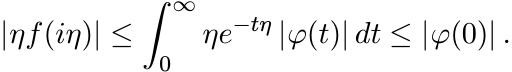 (0)
(0)
Hence, by Problem V.5.9 of MA, there exists a finite positive measure µ on ![]() such
that
such
that
(iv) Thus we have
(v) Compare the expression for f in (5.60) with the one obtained in (iv) and conclude
This is the assertion of Bochner’s theorem.
5.7 NOTES AND REFERENCES
Positive definite functions have applications in almost every area of modern analysis. In 1907 C. Carathéodory studied functions with power series
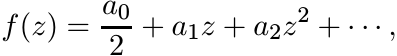
and found necessary and sufficient conditions on the sequence {an} in order that f maps the unit disk into the right half-plane. In 1911 O. Toeplitz observed that Carathéodory’s condition is equivalent to (5.1). The connection with Fourier series and transforms has been pointed out in this chapter. In probability theory positive definite functions arise as characteristic functions of various distributions. See E. Lukacs, Characteristic Functions, Griffin, 1960, and R. Cuppens, Decomposition of Multivariate Probabilities, Academic Press, 1975. We mention just one more very important area of their application: the theory of group representations.
Let G be a locally compact topological group. A (continuous) complex-valued function
φ on G is positive definite if for each N = 1, 2, . . . , the N × N matrix ![]() is positive
for every choice of elements g0, . . . , gN−1 from G. A unitary representation of
G is a homomorphism
is positive
for every choice of elements g0, . . . , gN−1 from G. A unitary representation of
G is a homomorphism ![]() from G into the group of unitary operators on a Hilbert space
H such that for every fixed
from G into the group of unitary operators on a Hilbert space
H such that for every fixed ![]() the map
the map ![]() from G into
from G into ![]() is continuous. (This is called
strong continuity.) It is easy to see that if Ug is a unitary representation of G
in the Hilbert space
is continuous. (This is called
strong continuity.) It is easy to see that if Ug is a unitary representation of G
in the Hilbert space ![]() , then for every
, then for every ![]() the function
the function
is positive definite on G. (This is a generalization of Exercise 5.6.1.) The converse
is an important theorem of Gelfand and Raikov proved in 1943. This says that for
every positive definite function φ on G there exist a Hilbert space ![]() , a unitary representation
Ug of G in
, a unitary representation
Ug of G in ![]() , and a vector
, and a vector ![]() such that the equation (5.61) is valid. This is one of
the first theorems in the representation theory of infinite groups. One of its corollaries
is that every locally compact group has sufficiently many irreducible unitary representations.
More precisely, for every element g of G different from the identity, there exists
an irreducible unitary representation of G for which Ug is not the identity operator.
such that the equation (5.61) is valid. This is one of
the first theorems in the representation theory of infinite groups. One of its corollaries
is that every locally compact group has sufficiently many irreducible unitary representations.
More precisely, for every element g of G different from the identity, there exists
an irreducible unitary representation of G for which Ug is not the identity operator.
An excellent survey of positive definite functions is given in J. Stewart, Positive definite functions and generalizations, an historical survey, Rocky Mountain J. Math., 6 (1976) 409–434. Among books, we recommend C. Berg, J.P.R. Christensen, and P. Ressel, Harmonic Analysis on Semigroups, Springer, 1984, and Z. Sasvári, Positive Definite and Definitizable Functions Akademie-Verlag, Berlin, 1994.
In Section 5.2 we have constructed a variety of examples using rather elementary arguments. These, in turn, are useful in proving that certain matrices are positive. The criterion in 5.2.15 is due to G. Pólya, Remarks on characteristic functions, Proc. Berkeley Symp. Math. Statist. & Probability, 1949, pp.115-123. This criterion is very useful as its conditions can be easily verified.
The ideas and results of Sections 5.2 and 5.3 are taken from the papers R. Bhatia and K. R. Parthasarathy, Positive definite functions and operator inequalities, Bull. London Math. Soc. 32 (2000) 214–228, H. Kosaki, Arithmetic-geometric mean and related inequalities for operators, J. Funct. Anal., 15 (1998) 429–451, F. Hiai and H. Kosaki, Comparison of various means for operators, ibid., 163 (1999) 300–323, and F. Hiai and H. Kosaki, Means for matrices and comparison of their norms, Indiana Univ. Math. J., 48 (1999) 899–936.
The proof of Theorem 5.3.1 given here is from R. Bhatia and K. B. Sinha, Derivations, derivatives and chain rules, Linear Algebra Appl., 302/303 (1999) 231–244. Theorem 5.3.3 was proved by K. Löwner (C. Loewner) in Über monotone Matrixfunctionen, Math. Z., 38 (1934) 177–216. Loewner then used this theorem to show that a function is operator monotone on the positive half-line if and only if it has an analytic continuation mapping the upper half-plane into itself. Such functions are characterized by certain integral representations, namely, f is operator monotone if and only if
 (5.62)
for some real numbers α and β with β ≥ 0, and a positive measure µ that makes the integral above convergent. The connection between positivity of Loewner matrices and complex functions is made via Carathéodory’s theorem (mentioned at the beginning of this section) and its successors. Following Loewner’s work operator monotonicity of particular examples such as 5.3.5–5.3.8 was generally proved by invoking the latter two criteria (analytic continuation or integral representation). The more direct proofs based on the positivity of Loewner matrices given here are from the 2000 paper of Bhatia and Parthasarathy.
The inequality (5.24) and the more general (5.28) were proved in R. Bhatia and C. Davis, More matrix forms of the arithmetic-geometric mean inequality, SIAM J. Matrix Anal. Appl., 14 (1993) 132–136. For the operator norm alone, the inequality (5.28) was proved by E. Heinz, Beiträge zur Störungstheorie der Spektralzerlegung, Math. Ann., 123 (1951) 415–438. The inequality (5.24) aroused considerable interest and several different proofs of it were given by various authors. Two of them, R. A. Horn, Norm bounds for Hadamard products and the arithmetic-geometric mean inequality for unitarily invariant norms, Linear Algebra Appl., 223/224 (1995) 355–361, and R. Mathias, An arithmetic-geometric mean inequality involving Hadamard products, ibid., 184 (1993) 71–78, observed that the inequality follows from the positivity of the matrix in (5.27). The papers by Bhatia-Parthasarathy and Kosaki cited above were motivated by extending this idea further. The two papers used rather similar arguments and obtained similar results. The program was carried much further in the two papers of Hiai and Kosaki cited above to obtain an impressive variety of results on means. The interested reader should consult these papers as well as the monograph F. Hiai and H. Kosaki, Means of Hilbert Space Operators, Lecture Notes in Mathematics Vol. 1820, Springer, 2003.
The theorems of Herglotz and Bochner concern the groups ![]() and
and ![]() . They were generalized
to locally compact abelian groups by A. Weil, by D. A. Raikov, and by A. Powzner,
in independent papers appearing almost together. Further generalizations (non-abelian
or non-locally compact groups) exist. The original proof of Bochner’s theorem appears
in S. Bochner, Vorlesungen über Fouriersche Integrale, Akademie-Verlag, Berlin,
1932. Several other proofs have been published. The one given in Section 5.5 is taken
from R. Goldberg, Fourier Transforms, Cambridge University Press, 1961, and that
in Section 5.6 from N. I. Akhiezer and I. M. Glazman, Theory of Linear Operators
in Hilbert Space, Dover, 1993 (reprint of original editions). A generalization to
distributions is given in L. Schwartz, Théorie des Distributions, Hermann, 1954.
. They were generalized
to locally compact abelian groups by A. Weil, by D. A. Raikov, and by A. Powzner,
in independent papers appearing almost together. Further generalizations (non-abelian
or non-locally compact groups) exist. The original proof of Bochner’s theorem appears
in S. Bochner, Vorlesungen über Fouriersche Integrale, Akademie-Verlag, Berlin,
1932. Several other proofs have been published. The one given in Section 5.5 is taken
from R. Goldberg, Fourier Transforms, Cambridge University Press, 1961, and that
in Section 5.6 from N. I. Akhiezer and I. M. Glazman, Theory of Linear Operators
in Hilbert Space, Dover, 1993 (reprint of original editions). A generalization to
distributions is given in L. Schwartz, Théorie des Distributions, Hermann, 1954.
Integral representations such as the one given by Bochner’s theorem are often viewed
as a part of “Choquet Theory.” Continuous positive definite functions φ(x) such that
φ(0) = 1 form a compact convex set; the family ![]() is the set of extreme points of this
convex set.
is the set of extreme points of this
convex set.
Exercise 5.6.1 is an adumbration of the connections between positive definite functions
and spectral theory of operators. A basic theorem of M. H. Stone in the latter subject
says that every unitary representation ![]() of R in a Hilbert space H is of the form
Ut = eitA for some (possibly unbounded) self-adjoint operator A. (The operator A
is bounded if and only if ||Ut − I|| → 0 as t → 0.) The theorems of Stone and Bochner
can be derived from each other. See M. Reed and B. Simon, Methods of Modern Mathematical
Physics, Vols. I, II, Academic Press, 1972, 1975, Chapters VIII, IX.
of R in a Hilbert space H is of the form
Ut = eitA for some (possibly unbounded) self-adjoint operator A. (The operator A
is bounded if and only if ||Ut − I|| → 0 as t → 0.) The theorems of Stone and Bochner
can be derived from each other. See M. Reed and B. Simon, Methods of Modern Mathematical
Physics, Vols. I, II, Academic Press, 1972, 1975, Chapters VIII, IX.
A sequence ![]() is of positive type if for every positive integer N, we have
is of positive type if for every positive integer N, we have
 (5.63)
for every finite sequence of complex numbers ξ0, ξ1, . . . , ξN−1. This is equivalent to the requirement that for each N = 1, 2, . . . , the N × N matrix
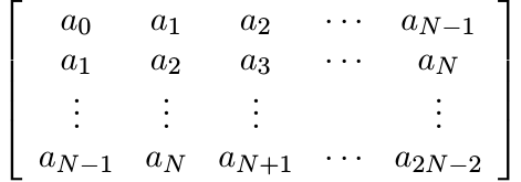 (5.64)
is positive. Compare these conditions with (5.1) and (5.2). (Matrices of the form (5.64) are called Hankel matrices while those of the form (5.2) are Toeplitz matrices.) A complex valued function φ on the positive half-line [0, ∞) is of positive type if for each N the N × N matrix
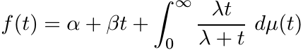
is positive for every choice of x0, . . . , xN−1 in [0, ∞). A theorem of Bernstein and Widder says that φ is of positive type if and only if there exists a positive measure µ on [0, ∞) such that
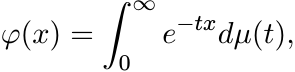 (5.66)
i.e., φ is the Laplace transform of a positive measure µ. Such functions are characterized also by being completely monotone, which, by definition, means that
See MA p.148 for the connection such functions have with operator monotone functions. The book of Berg, Christensen, and Ressel cited above is a good reference for the theory of these functions.
Our purpose behind this discussion is to raise a question. Suppose f is a function
mapping [0, ∞) into itself. Say that f is in the class ![]() if for each N the matrix
if for each N the matrix
is positive for every choice λ1, . . . , λN in [0, ∞). The class ![]() is precisely the
operator monotone functions. Is there a good characterisation of functions in
is precisely the
operator monotone functions. Is there a good characterisation of functions in ![]() ?
One can easily see that if
?
One can easily see that if ![]() , then so does 1/f. It is known that
, then so does 1/f. It is known that ![]() is contained in
is contained in
![]() ; see, e.g., M. K. Kwong, Some results on matrix monotone functions, Linear Algebra
Appl., 118 (1989) 129–153. (It is easy to see, using the positivity of the Cauchy
matrix, that for every λ > 0 the function g(t) = λt/(λ + t) is in
; see, e.g., M. K. Kwong, Some results on matrix monotone functions, Linear Algebra
Appl., 118 (1989) 129–153. (It is easy to see, using the positivity of the Cauchy
matrix, that for every λ > 0 the function g(t) = λt/(λ + t) is in ![]() . The integral
representation (5.62) then shows that every function in
. The integral
representation (5.62) then shows that every function in ![]() is in
is in ![]() .)
.)
The conjecture stated after Exercise 5.6.3 goes back to D. Bessis, P. Moussa, and
M. Villani, Monotonic converging variational approximations to the functional integrals
in quantum statistical mechanics, J. Math. Phys., 16 (1975) 2318–2325. A more recent
report on the known partial results may be found in P. Moussa, On the representation
of Tr ![]() as a Laplace transform, Rev. Math. Phys., 12 (2000) 621–655. E. H. Lieb and
R. Seiringer, Equivalent forms of the Bessis-Moussa-Villani conjecture, J. Stat.
Phys., 115 (2004) 185–190, point out that the statement of this conjecture is equivalent
to the following: for all A and B positive, and all natural numbers p, the polynomial
as a Laplace transform, Rev. Math. Phys., 12 (2000) 621–655. E. H. Lieb and
R. Seiringer, Equivalent forms of the Bessis-Moussa-Villani conjecture, J. Stat.
Phys., 115 (2004) 185–190, point out that the statement of this conjecture is equivalent
to the following: for all A and B positive, and all natural numbers p, the polynomial
![]() has only positive coefficients. When this polynomial is multiplied out, the co-efficient
of λr is a sum of terms each of which is the trace of a word in A and B. It has been
shown by C. R. Johnson and C. J. Hillar, Eigenvalues of words in two positive definite
letters, SIAM J. Matrix Anal. Appl., 23 (2002) 916-928, that some of the individual
terms in this sum can be negative. For example, tr A2B2AB can be negative even when
A and B are positive.
has only positive coefficients. When this polynomial is multiplied out, the co-efficient
of λr is a sum of terms each of which is the trace of a word in A and B. It has been
shown by C. R. Johnson and C. J. Hillar, Eigenvalues of words in two positive definite
letters, SIAM J. Matrix Anal. Appl., 23 (2002) 916-928, that some of the individual
terms in this sum can be negative. For example, tr A2B2AB can be negative even when
A and B are positive.
The matrix Z in Exercise 5.6.7 was studied by M. K. Kwong, On the definiteness of the solutions of certain matrix equations, Linear Algebra Appl., 108 (1988) 177–197. It was shown here that for each n ≥ 2, there exists a number tn such that Z is positive for all t in (−2, tn], and further tn > 2 for all n, tn = ∞, 8, 4 for n = 2, 3, 4, respectively. The complete solution (given in Exercise 5.6.7) appears in the 2000 paper of Bhatia-Parthasarathy cited earlier. The idea and the method are carried further in R. Bhatia and D. Drissi, Generalised Lyapunov equations and positive definite functions, SIAM J. Matrix Anal. Appl., 27 (2005) 103-295–114. Using a Fourier transforms argument D. Drissi, Sharp inequalities for some operator means, preprint 2006, has shown that the function f(x) = (x cosh α x)/ sinh x is not positive definite when |α| > 1/2. The result of Exercise 5.6.9 is due to E. Andruchow, G. Corach, and D. Stojanoff, Geometric operator inequalities, Linear Algebra Appl., 258 (1997) 295-310, where other related inequalities are also discussed. The result of Exercise 5.6.10 was proved by D. K. Jocić, Cauchy-Schwarz and means inequalities for elementary operators into norm ideals, Proc. Am. Math. Soc., 126 (1998) 2705–2711. Cognate results are proved in D. K. Jocić, Cauchy-Schwarz norm inequalities for weak∗-integrals of operator valued functions, J. Funct. Anal., 218 (2005) 318–346.
Proposition 5.6.11 is proved in the Hiai-Kosaki papers cited earlier. They also give an example of two means where M1 ≤ M2, but M1 << M2 is not true. The simple example in Exercise 5.6.12 is from R. Bhatia, Interpolating the arithmetic-geometric mean inequality and its operator version, Linear Algebra Appl., 413 (2006) 355–363.
Conditionally positive definite matrices are discussed in Chapter 4 of the book R.
B. Bapat and T. E. S. Raghavan, Nonnegative Matrices and Applications, Cambridge
University Press, 1997, and more briefly in Section 6.3 of R. A. Horn and C. R. Johnson,
Topics in Matrix Analysis, Cambridge University Press, 1991. This section also contains
a succinct discussion of infinitely divisible matrices and references to original
papers. The results of Exercises 5.6.20 and 5.6.21 are taken from R. Bhatia, Infinitely
divisible matrices, Am. Math. Monthly, 113 (2006) 221–235, and those of Exercises
5.6.23, 5.6.24 and 5.6.25 from R. Bhatia and H. Kosaki, Mean matrices and infinite
divisibility, preprint 2006. In this paper it is shown that for several classes
of means m(a, b), matrices of the form [[m(λi, λj)]] are infinitely divisible if
![]() for all a and b; and if
for all a and b; and if ![]() , then matrices of the form [[1/m(λi, λj)]] are infinitely
divisible. The contents of Exercise 5.6.28 are taken from H. Kosaki, On infinite
divisibility of positive definite functions, preprint 2006. In this paper Kosaki
uses very interesting ideas from complex analysis to obtain criteria for infinite
divisibility.
, then matrices of the form [[1/m(λi, λj)]] are infinitely
divisible. The contents of Exercise 5.6.28 are taken from H. Kosaki, On infinite
divisibility of positive definite functions, preprint 2006. In this paper Kosaki
uses very interesting ideas from complex analysis to obtain criteria for infinite
divisibility.
We have spoken of Loewner’s theorems that say that the Loewner matrices associated with a function f on [0, ∞) are positive if and only if f has an analytic continuation mapping the upper half-plane into itself. R. A. Horn, On boundary values of a schlicht mapping, Proc. Am. Math. Soc., 18 (1967) 782–787, showed that this analytic continuation is a one-to-one (schlicht) mapping if and only if the Loewner matrices associated with f are infinitely divisible. This criterion gives another proof of the infinite divisibility of the matrices in Sections 5.3.5 and 5.3.7.
Infinitely divisible distribution functions play an important role in probability theory. These are exactly the limit distributions for sums of independent random variables. See, for example, L. Breiman, Probability, Addison-Wesley, 1968, pp. 190–196, or M. Loeve, Probability Theory, Van Nostrand, 1963, Section 22. The two foundational texts on this subject are B. V. Gnedenko and A. N. Kolmogorov, Limit Distributions for Sums of Independent Random Variables, Addison-Wesley, 1954, and P. Lévy, Théorie de l’ Addition des Variables Aléatoires, Gauthier-Villars, 1937. The famous LévyKhintchine Formula says that a continuous positive definite function φ, with φ(0) = 1, is infinitely divisible if and only if it can be represented as
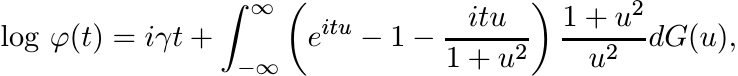
where γ is a real number, G is a nondecreasing function of bounded variation, and the integrand at u = 0 is to be interpreted as the limiting value −t2/2. This representation of log f(t) is unique. See the book by Gnedenko and Kolmogorov, p. 76. A list of such representations for some of the examples we have considered is given in Lukacs, p. 93.
A positive definite function is said to be self-decomposable if for every real number ν in (0, 1) there exists a positive definite function φν such that
Such functions are of importance in probability theory; see Section 23.3 of Loeve’s book. It is shown there that if φ is self-decomposable, then it is infinitely divisible, and so are the functions φν, 0 < ν < 1. Our discussion in Section 5.2.10 shows that the functions 1/(1 + x2), 1/cosh x and x/sinh x are self-decomposable. So, the infinite divisibility of some of the functions in Exercises 5.6.22–5.6.28 is a consequence also of Loeve’s theorem.
In Exercise 5.6.28 we observed that if a ≥ b ≥ 0, then the function f(x) = (1 + bx2)/(1 + ax2) is infinitely divisible, and in Exercise 5.6.29 asked the reader to use this to show that g(x) = (tanh x)/x is infinitely divisible. In the paper Z. J. Jurek and M. Yor, Self decomposable laws associated with hyperbolic functions, Probability and Mathematical Statistics, 24 (2004), 181–190, it is observed that the function f is not self-decomposable but the function g is. Some of the results in H. Kosaki, On infinite divisibility of positive definite functions, preprint 2006, can be rephrased to say that certain functions are self-decomposable. His list includes, for example, 1/(cosh x + a), −1 ≤ a ≤ 1. The relevance and importance of these functions in probability theory is explained in the paper of Jurek and Yor, and in the references therein.
Finally, we make a few comments on operator inequalities with special reference to the arithmetic-geometric mean inequality. Operator inequalities are sought and found in three different versions. If A and B are positive, we may have sometimes an inequality A ≥ B. By Weyl’s monotonicity principle, this implies that λj(A) ≥ λj(B), 1 ≤ j ≤ n, where λj(A) is the jth eigenvalue of A counted in decreasing order. (This is equivalent to the existence of a unitary matrix U such that A ≥ UBU∗.) This, in turn implies that |||A||| ≥ |||B||| for all unitarily invariant norms. If A and B are not positive, we may ask whether |A| ≥ |B|. This implies the set of inequalities sj(A) ≥ sj(B) for all the singular values, which in turn implies |||A||| ≥ |||B||| for all unitarily invariant norms.
In Chapter 4 we saw an arithmetic-geometric mean inequality of the first kind; viz.,
![]() for any two positive matrices. The inequality (5.23) and its stronger version (5.24)
are of the third kind. An inequality of the second kind was proved by R. Bhatia and
F. Kittaneh, On the singular values of a product of operators, SIAM J. Matrix Anal.
Appl., 11 (1990) 272–277. This says that
for any two positive matrices. The inequality (5.23) and its stronger version (5.24)
are of the third kind. An inequality of the second kind was proved by R. Bhatia and
F. Kittaneh, On the singular values of a product of operators, SIAM J. Matrix Anal.
Appl., 11 (1990) 272–277. This says that ![]() , for 1 ≤ j ≤ n. This inequality for singular
values implies the inequality (5.23) for norms. A stronger version sj(A1/2XB1/2)
≤ sj(AX + XB)/2 is not always true. So, there is no second level inequality generalising
(5.24).
, for 1 ≤ j ≤ n. This inequality for singular
values implies the inequality (5.23) for norms. A stronger version sj(A1/2XB1/2)
≤ sj(AX + XB)/2 is not always true. So, there is no second level inequality generalising
(5.24).
For positive numbers a and b, the arithmetic-geometric mean inequality may be written in three different ways:
(i)
![]() ,
,
(ii)
![]() ,
,
(iii)
![]() .
.
While each of these three may be obtained from the other, the matrix versions suggested by them are different. For example (i) leads to the question whether
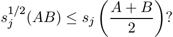
This is different from the inequality of Bhatia and Kittaneh stated above. It is not known whether this is true when n > 2. Weaker than this is the third-level inequality
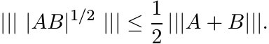
This too is known to be true for a large class of unitarily invariant norms (including Schatten p-norms for p = 1 and for p ≥ 2). It is not known whether it is true for all unitarily invariant norms. From properties of the matrix square function, one can see that this last (unproven) inequality is stronger than the assertion
This version of the arithmetic-geometric mean inequality is known to be true. Thus there are quite a few subtleties involved in noncommutative versions of simple inequalities. A discussion of some of these matters may be found in R. Bhatia and F. Kittaneh, Notes on matrix arithmetic-geometric mean inequalities, Linear Algebra Appl., 308 (2000) 203–211, where the results just mentioned are proved. We recommend the monograph X. Zhan, Matrix Inequalities, Lecture Notes in Mathematics Vol. 1790, Springer, 2002 for a discussion of several topics related to these themes.