
Chapter Two
Positive Linear Maps
In this chapter we study linear maps on spaces of matrices. We use the symbol Φ for
a linear map from ![]() into
into ![]() . When k = 1 such a map is called a linear functional, and
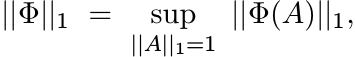
we use the lower-case symbol φ for it. The norm of Φ is
. When k = 1 such a map is called a linear functional, and
we use the lower-case symbol φ for it. The norm of Φ is
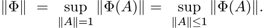
In general, it is not easy to calculate this. One of the principal results of this
chapter is that if Φ carries positive elements of ![]() to positive elements of
to positive elements of ![]() , then
||Φ|| = ||Φ(I)||.
, then
||Φ|| = ||Φ(I)||.
2.1 REPRESENTATIONS
The interplay between algebraic properties of linear maps Φ and their metric properties
is best illustrated by considering representations of ![]() in
in ![]() . These are linear maps
that
. These are linear maps
that
(i) preserve products; i.e., Φ(AB) = Φ(A)Φ(B);
(ii) preserve adjoints; i.e., Φ(A∗) = Φ(A)∗;
(iii) preserve the identity; i.e., Φ(I) = I.
Let σ(A) denote the spectrum of A, and spr(A) its spectral radius.
2.1.1 Exercise
If Φ has properties (i) and (iii), then
Hence
Our norm || · || has two special properties related to the ∗ operation: ||A||2 = ||A∗A||; and ||A|| = spr(A) if A is Hermitian. So, if Φ is a representation we have
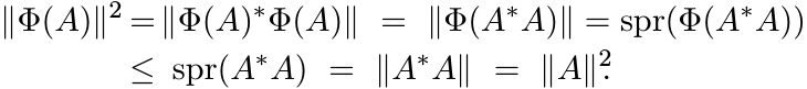
Thus ||Φ(A)|| ≤ ||A|| for all A. Since Φ(I) = I, we have ||Φ|| = 1.
We have shown that every representation has norm one.
How does one get representations? For each unitary element of Mn, Φ(A) = U∗AU is
a representation. Direct sums of such maps are representations; i.e., if U1, . .
. , Ur are n × n unitary matrices, then ![]() is a representation.
is a representation.
Choosing Uj = I, 1 ≤ j ≤ r, we get the representation Φ(A) = ![]() . The operator
. The operator ![]() is unitarily
equivalent to
is unitarily
equivalent to ![]() , and
, and ![]() is another representation.
is another representation.
2.1.2 Exercise
All representations of ![]() are obtained by composing unitary conjugations and tensor
products with Ir, r = 1, 2, . . .. Thus we have exhausted the family of representations
by the examples we saw above. [Hint: A representation carries orthogonal projections
to orthogonal projections, unitaries to unitaries, and preserves unitary conjugation.]
are obtained by composing unitary conjugations and tensor
products with Ir, r = 1, 2, . . .. Thus we have exhausted the family of representations
by the examples we saw above. [Hint: A representation carries orthogonal projections
to orthogonal projections, unitaries to unitaries, and preserves unitary conjugation.]
Thus the fact that ||Φ|| = 1 for every representation Φ is not too impressive; we
do know ![]() and ||U∗AU|| = ||A||.
and ||U∗AU|| = ||A||.
We will see how we can replace the multiplicativity condition (i) by less restrictive conditions and get a richer theory.
2.2 POSITIVE MAPS
A linear map ![]() is called positive if Φ(A) ≥ O whenever A ≥ O. It is said to be unital
if Φ(I) = I. We will say Φ is strictly positive if Φ(A) > O whenever A > O.
It is easy to see that a positive linear map Φ is strictly positive if and only if
Φ(I) > O.
is called positive if Φ(A) ≥ O whenever A ≥ O. It is said to be unital
if Φ(I) = I. We will say Φ is strictly positive if Φ(A) > O whenever A > O.
It is easy to see that a positive linear map Φ is strictly positive if and only if
Φ(I) > O.
2.2.1 Examples
(i)
φ(A) = trA is a positive linear functional; ![]() is positive and unital.
is positive and unital.
(ii)
Every linear functional on Mn has the form φ(A) = trAX for some ![]() . It is easy to see
that φ is positive if and only if X is a positive matrix; φ is unital if trX = 1.
(Positive matrices of trace one are called density matrices in the physics literature.)
. It is easy to see
that φ is positive if and only if X is a positive matrix; φ is unital if trX = 1.
(Positive matrices of trace one are called density matrices in the physics literature.)
(iii)
Let ![]() , the sum of all entries of A. If e is the vector with all of its entries equal
to one, and E = ee∗, the matrix with all entries equal to one, then
, the sum of all entries of A. If e is the vector with all of its entries equal
to one, and E = ee∗, the matrix with all entries equal to one, then
Thus φ is a positive linear functional.
(iv)
The map ![]() is a positive map of
is a positive map of ![]() into itself. (Its range consists of scalar matrices.)
into itself. (Its range consists of scalar matrices.)
(v) Let Atr denote the transpose of A. Then the map Φ(A) = Atr is positive.
(vi)
Let X be an n × k matrix. Then Φ(A) = X∗AX is a positive map from ![]() into
into ![]() .
.
(vii) A special case of this is the compression map that takes an n× n matrix to a k × k block in its top left corner.
(viii)
Let P1, . . . , Pr be mutually orthogonal projections with ![]() Pr = I. The operator
Pr = I. The operator
![]() is called a pinching of A. In an appropriate coordinate system this can be described
as
is called a pinching of A. In an appropriate coordinate system this can be described
as
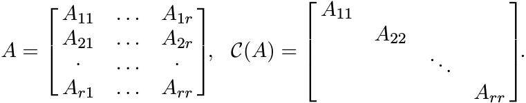
Every pinching is positive. A special case of this is r = n and each Pj is the projection onto the linear span of the basis vector ej. Then C(A) is the diagonal part of A.
(ix)
Let B be any positive matrix. Then the map ![]() is positive. So is the map Φ(A) = A ◦
B.
is positive. So is the map Φ(A) = A ◦
B.
(x)
Let A be a matrix whose spectrum is contained in the open right half plane. Let LA(X)
= A∗X + XA. The operator LA on ![]() is invertible and its inverse
is invertible and its inverse ![]() is a positive linear
map. (See the discussion in Exercise 1.2.10.)
is a positive linear
map. (See the discussion in Exercise 1.2.10.)
(xi) Any positive linear combination of positive maps is positive. Any convex combination of positive unital maps is positive and unital.
It is instructive to think of positive maps as noncommutative (matrix) averaging operations. Let C(X) be the space of continuous functions on a compact metric space. Let φ be a linear functional on C(X). By the Riesz representation theorem, there exists a signed measure µ on X such that
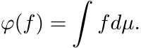 (2.3)
(2.3)The linear functional φ is called positive if φ(f) ≥ 0 for every (pointwise) nonnegative function f. For such a φ, the measure µ representing it is a positive measure. If φ maps the function f ≡ 1 to the number 1, then φ is said to be unital, and then µ is a probability measure. The integral (2.3) is then written as
and called the expectation of f. Every positive, unital, linear functional on C(X) is an expectation (with respect to a probability measure µ). A positive, unital, linear map Φ may thus be thought of as a noncommutative analogue of an expectation map.
2.3 SOME BASIC PROPERTIES OF POSITIVE MAPS
We prove three theorems due to Kadison, Choi, and Russo and Dye. Our proofs use 2 × 2 block matrix arguments.
2.3.1 Lemma
Every positive linear map is adjoint-preserving; i.e., Φ(T∗) = Φ(T)∗ for all T.
Proof. First we show that Φ(A) is Hermitian if A is Hermitian. Every Hermitian matrix A has a Jordan decomposition
So,
is the difference of two positive matrices, and is therefore Hermitian. Every matrix T has a Cartesian decomposition
So,
2.3.2 Theorem ( Kadison’s Inequality)
Let Φ be positive and unital. Then for every Hermitian A
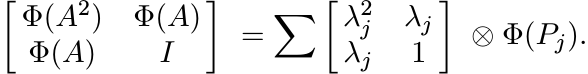
Proof. By the spectral theorem, ![]() , where λj are the eigenvalues of A and Pj the corresponding
projections with
, where λj are the eigenvalues of A and Pj the corresponding
projections with ![]() . Then
. Then ![]() and
and
Since Pj are positive, so are Φ(Pj). Therefore,
Each summand in the last sum is positive and, hence, so is the sum. By Theorem 1.3.3, therefore,
2.3.3 Exercise
The inequality (2.5) may not be true if Φ is not unital.
Recall that for real functions we have (Ef)2 ≤ Ef2. The inequality (2.5) is a noncommutative
version of this. It should be pointed out that not all inequalities for expectations
of real functions have such noncommutative counterparts. For example, we do have
(Ef)4 ≤ Ef4, but the analogous inequality Φ(A)4 ≤ Φ(A4) is not always true. To see
this, let Φ be the compression map from ![]() to
to ![]() , taking a 3 × 3 matrix to its top left
2 × 2 submatrix. Let
, taking a 3 × 3 matrix to its top left
2 × 2 submatrix. Let
Then ![]() and
and ![]() .
.
This difference can be attributed to the fact that while the function f(t) = t4 is convex on the real line, the matrix function f(A) = A4 is not convex on Hermitian matrices.
The following theorem due to Choi generalizes Kadison’s inequality to normal operators.
2.3.4 Theorem (Choi)
Let Φ be positive and unital. Then for every normal matrix A
Proof. The proof is similar to the one for Theorem 2.3.2. We have
So
is positive. ■
In Chapter 3, we will see that the condition that A be normal can be dropped if we impose a stronger condition (2-positivity) on Φ.
2.3.5 Exercise
If A is normal, then Φ(A) need not be normal. Thus the left-hand sides of the two inequalities (2.6) can be different.
2.3.6 Theorem (Choi’s Inequality)
Let Φ be strictly positive and unital. Then for every strictly positive matrix A
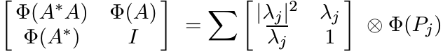
Proof. The proof is again similar to that of Theorem 2.3.2. Now we have ![]() with λj
> 0. Then
with λj
> 0. Then ![]() , and
, and
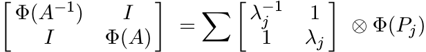
is positive. Hence, by Theorem 1.3.3
2.3.7 Theorem (The Russo-Dye Theorem)
If Φ is positive and unital, then ||Φ|| = 1.
Proof. We show first that ||Φ(U)|| ≤ 1 when U is unitary. In this case the eigenvalues
λj are complex numbers of modulus one. So, from the spectral resolution ![]() , we get
, we get
Hence, by Proposition 1.3.1, ||Φ(U)|| ≤ 1. Now if A is any contraction, then we can
write ![]() where U, V are unitary. (Use the singular value decomposition of A and observe
that if 0 ≤ s ≤ 1, then we have
where U, V are unitary. (Use the singular value decomposition of A and observe
that if 0 ≤ s ≤ 1, then we have ![]() for some θ.) So
for some θ.) So

Thus ||Φ|| ≤ 1, and since Φ is unital ||Φ|| = 1. ■
Second proof. Let ||A|| ≤ 1. Then A has a unitary dilation Â
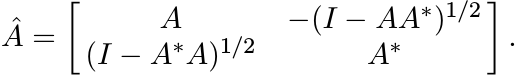 (2.8)
(2.8)(Check that this is a unitary element of M2n.)
Now let Ψ be the compression map taking a 2n × 2n matrix to its top left n × n corner. Then Ψ is positive and unital. So, the composition Φ ◦ Ψ is positive and unital. Now Choi’s inequality (2.6) can be used to get
But this says
This shows that ||Φ(A)|| ≤ 1 whenever ||A|| ≤ 1. Hence, ||Φ|| = 1. ■
We can extend the result to any positive linear map as follows.
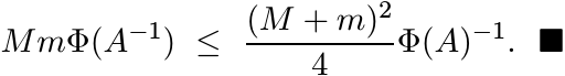
2.3.8 Corollary
Let Φ be a positive linear map. Then ||Φ|| = ||Φ(I)||.
Proof. Let P = Φ(I), and assume first that P is invertible. Let
Then Ψ is a positive unital linear map. So, we have
Thus ||Φ|| ≤ ||P||; and since Φ(I) = P, we have ||Φ|| = ||P||. This proves the assertion when Φ(I) is invertible. The general case follows from this by considering the family Φε(A) = Φ(A) + εI and letting ε ↓ 0. ■
The assertion of (this Corollary to) the Russo-Dye theorem is some times phrased
as: every positive linear map on ![]() attains its norm at the identity matrix.
attains its norm at the identity matrix.
2.3.9 Exercise
There is a simpler proof of this theorem in the case of positive linear functionals. In this case φ(A) = trAX for some positive matrix X. Then
Here ||T||1 is the trace norm of T defined as ||T||1 = s1(T)+· · ·+sn(T). The inequality above is a consequence of the fact that this norm is the dual of the norm || · ||.
2.4 SOME APPLICATIONS
We have seen several examples of positive maps. Using the Russo-Dye Theorem we can calculate their norms easily. Thus, for example,
for every pinching of A. (This can be proved in several ways. See MA pp. 50, 97.)
If A is positive, then the Schur multiplier SA is a positive map. So,
This too can be proved in many ways. We have seen this before in Theorem 1.4.1.
We have discussed the Lyapunov equation
where A is an operator whose spectrum is contained in the open right half plane.
(Exercise 1.2.10, Example 2.2.1 (x)). Solving this equation means finding the inverse
of the Lyapunov operator LA defined as LA(X) = A∗X + XA. We have seen that ![]() is a
positive linear map. In some situations W is known with some imprecision, and we
have the perturbed equation
is a
positive linear map. In some situations W is known with some imprecision, and we
have the perturbed equation
If X and X+ΔX are the solutions to (2.11) and (2.12), respectively, one wants to find bounds for ||ΔX||. This is a very typical problem in numerical analysis. Clearly,
Since ![]() is positive we have
is positive we have ![]() . This simplifies the problem considerably. The same considerations
apply to the Stein equation (Exercise 1.2.11).
. This simplifies the problem considerably. The same considerations
apply to the Stein equation (Exercise 1.2.11).
Let ![]() be the k-fold tensor product
be the k-fold tensor product ![]() and let
and let ![]() be the k-fold product
be the k-fold product ![]() of an operator
A on
of an operator
A on ![]() . For 1 ≤ k ≤ n, let
. For 1 ≤ k ≤ n, let ![]() be the subspace of
be the subspace of ![]() spanned by antisymmetric tensors.
This is called the antisymmetric tensor product, exterior product, or Grassmann product.
The operator
spanned by antisymmetric tensors.
This is called the antisymmetric tensor product, exterior product, or Grassmann product.
The operator ![]() leaves this space invariant and the restriction of
leaves this space invariant and the restriction of ![]() to it is denoted
as ∧kA. This is called the kth Grassmann power, or the exterior power of A.
to it is denoted
as ∧kA. This is called the kth Grassmann power, or the exterior power of A.
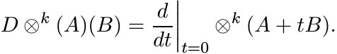
Consider the map ![]() . The derivative of this map at A, denoted as
. The derivative of this map at A, denoted as ![]() , is a linear map
from
, is a linear map
from ![]() into
into ![]() . Its action is given as
. Its action is given as
Hence,
It follows that
We want to find an expression for ||D ∧k (A)||.
Recall that ∧k is multiplicative, ∗ - preserving, and unital (but not linear!). Let A = USV be the singular value decomposition of A. Then
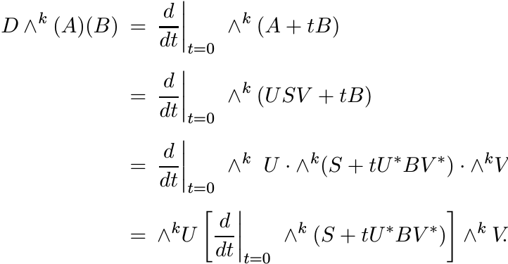
Thus
and hence
Thus to calculate ||D ∧k (A)||, we may assume that A is positive and diagonal.
Now note that if A is positive, then for every positive B, the expression (2.13)
is positive. So ![]() is a positive linear map from
is a positive linear map from ![]() into
into ![]() . The operator D ∧k (A)(B) is
the restriction of (2.13) to the invariant subspace
. The operator D ∧k (A)(B) is
the restriction of (2.13) to the invariant subspace ![]() . So ∧k(A) is also a positive
linear map. Hence
. So ∧k(A) is also a positive
linear map. Hence
Let A = diag(s1, . . . , sn) with s1 ≥ s2 ≥ · · · ≥ sn ≥ 0. Then ∧kA is a diagonal
matrix of size ![]() whose diagonal entries are si1si2 · · · sik, 1 ≤ i1 < i2 <
· · · < ik ≤ n. Use this to see that
whose diagonal entries are si1si2 · · · sik, 1 ≤ i1 < i2 <
· · · < ik ≤ n. Use this to see that
the elementary symmetric polynomial of degree k − 1 with arguments s1, . . . , sk.
The effect of replacing D ∧k (A)(B) by D ∧k (A)(I) is to reduce a highly noncommutative problem to a simple commutative one. Another example of this situation is given in Section 2.7.
2.5 THREE QUESTIONS
Let ![]() be a linear map. We have seen that if Φ is positive, then
be a linear map. We have seen that if Φ is positive, then
Clearly, this is a useful and important theorem. It is natural to explore how much, and in what directions, it can be extended.
Question 1 Are there linear maps other than positive ones for which (2.16) is true? In other words, if a linear map Φ attains its norm at the identity, then must Φ be positive?
Before attempting an answer, we should get a small irritant out of the way. If the condition (2.16) is met by Φ, then it is met by −Φ also. Clearly, both of them cannot be positive maps. So assume Φ satisfies (2.16) and
2.5.1 Exercise
If k = 1, the answer to our question is yes. In this case φ(A) = trAX for some X. Then ||φ|| = ||X||1 (see Exercise 2.3.9). So, if φ satisfies (2.16) and (2.17), then ||X||1 = trX. Show that this is true if and only if X is positive. Hence φ is positive.
If k ≥ 2, this is no longer true. For example, let Φ be the linear map on ![]() defined
as
defined
as
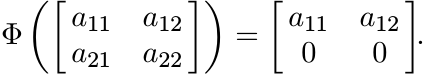
Then ||Φ|| = ||Φ(I)|| = 1 and Φ(I) ≥ O, but Φ is not positive.
It is a remarkable fact that if Φ is unital and ||Φ|| = 1, then Φ is positive. Thus supplementing (2.16) with the condition Φ(I) = I ensures that Φ is positive. This is proved in the next section.
Question 2 Let S be a linear subspace of ![]() and let
and let ![]() be a linear map. Do we still have
a theorem like the Russo-Dye theorem? In other words how crucial is the fact that
the domain of Φ is Mn (or possibly a subalgebra)?
be a linear map. Do we still have
a theorem like the Russo-Dye theorem? In other words how crucial is the fact that
the domain of Φ is Mn (or possibly a subalgebra)?
Again, for the question to be meaningful, we have to demand of S a little more structure. If we want to talk of positive unital maps, then S must contain some positive elements and I.
2.5.2 Definition
A linear subspace S of ![]() is called an operator system if it is ∗ closed (i.e., if
A ∈ S, then A∗ ∈ S ) and contains I.
is called an operator system if it is ∗ closed (i.e., if
A ∈ S, then A∗ ∈ S ) and contains I.
Let S be an operator system. We want to know whether a positive linear map ![]() attains
its norm at I. The answer is yes if k = 1, and no if k ≥ 2. However, we do have ||Φ||
≤ 2||Φ(I)|| for all k.
attains
its norm at I. The answer is yes if k = 1, and no if k ≥ 2. However, we do have ||Φ||
≤ 2||Φ(I)|| for all k.
A related question is the following:
Question 3 By the Hahn-Banach theorem, every linear functional φ on (a linear subspace)
S can be extended to a linear functional ![]() on
on ![]() in such a way that
in such a way that ![]() . Now we are considering
positivity rather than norms. So we may ask whether a positive linear functional
φ on an operator system S in
. Now we are considering
positivity rather than norms. So we may ask whether a positive linear functional
φ on an operator system S in ![]() can be extended to a positive linear functional
can be extended to a positive linear functional ![]() on
on
![]() . The answer is yes. This is called the Krein extension theorem. Then since
. The answer is yes. This is called the Krein extension theorem. Then since ![]() , we
have ||φ|| = φ(I).
, we
have ||φ|| = φ(I).
Next we may ask whether a positive linear map Φ from ![]() into
into ![]() can be extended to a
positive linear map
can be extended to a
positive linear map ![]() from
from ![]() into
into ![]() . If this were the case, then we would have ||Φ||
= ||Φ(I)||. But we have said that this is not always true when k ≥ 2. This is illustrated
by the following example.
. If this were the case, then we would have ||Φ||
= ||Φ(I)||. But we have said that this is not always true when k ≥ 2. This is illustrated
by the following example.
2.5.3 Example
Let n be any number bigger than 2 and let S be the n×n permutation matrix
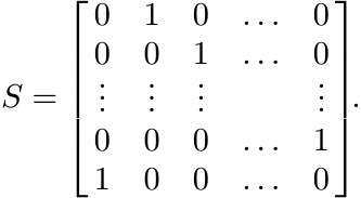
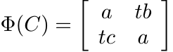
Let S be the collection of all matrices C of the form C = aI+bS+cS∗, a, b, c ∈ ![]() .
(The matrices C are circulant matrices.) Then
.
(The matrices C are circulant matrices.) Then ![]() is an operator system in
is an operator system in ![]() . What are
the positive elements of
. What are
the positive elements of ![]() ? First, we must have a ≥ 0 and
? First, we must have a ≥ 0 and ![]() . The eigenvalues of S are
1, ω, . . . , ωn−1, the n roots of 1. So, the eigenvalues of C are
. The eigenvalues of S are
1, ω, . . . , ωn−1, the n roots of 1. So, the eigenvalues of C are
and C is positive if and only if all these numbers are nonnegative.
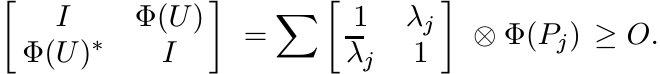
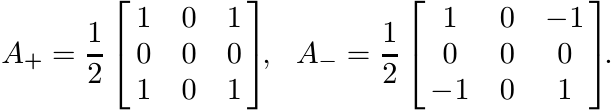
It is helpful to consider the special case n = 4. The fourth roots of unity are {1, i, −1, −i} and one can see that a matrix C of the type above is positive if and only if
Let ![]() be the map defined as
be the map defined as
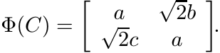
Then Φ is linear, positive, and unital. Since
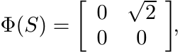
![]() . So, Φ cannot be extended to a positive, linear, unital map from
. So, Φ cannot be extended to a positive, linear, unital map from ![]() into
into ![]() .
.
2.5.4 Exercise
Let n ≥ 3 and consider the operator system ![]() defined in the example above. For every
t the map
defined in the example above. For every
t the map ![]() defined as
defined as
is linear and unital. Show that for 1 < t < 2 there exists an n such that the map Φ is positive.
We should remark here that the elements of ![]() commute with each other (though, of course,
commute with each other (though, of course,
![]() is not a subalgebra of
is not a subalgebra of ![]() ).
).
In the next section we prove the statements that we have made in answer to the three questions.
2.6 POSITIVE MAPS ON OPERATOR SYSTEMS
Let ![]() be an operator system in
be an operator system in ![]() . the set of self-adjoint elements of
. the set of self-adjoint elements of ![]() , and
, and ![]() the set
of positive elements in it.
the set
of positive elements in it.
Some of the operations that we performed freely in ![]() may take us outside
may take us outside ![]() . Thus if
. Thus if
![]() , then Re
, then Re ![]() and Im T =
and Im T = ![]() are in
are in ![]() . However, if
. However, if ![]() , then the positive and negative parts
A± in the Jordan decomposition of A need not be in
, then the positive and negative parts
A± in the Jordan decomposition of A need not be in ![]() . For example, consider
. For example, consider
This is an operator system. The matrix ![]() is in
is in ![]() . Its Jordan components are
. Its Jordan components are
They do not belong to S.
However, it is possible still to write every Hermitian element A of ![]() as
as
Just choose
 (2.19)
Thus we can write every ![]() as
as
Using this decomposition we can prove the following lemma.
2.6.1 Lemma
Let Φ be a positive linear map from an operator system ![]() into
into ![]() . Then Φ(T∗) = Φ(T)∗
for all
. Then Φ(T∗) = Φ(T)∗
for all ![]() .
.
2.6.2 Exercise
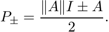
If A = P1 − P2 where P1, P2 are positive, then
2.6.3 Theorem
Let Φ be a positive linear map from an operator system ![]() into
into ![]() . Then
. Then
and
(Thus if Φ is also unital, then ||Φ|| = 1 on the space ![]() , and ||Φ|| ≤ 2 on
, and ||Φ|| ≤ 2 on ![]() .)
.)
Proof. If P is a positive element of ![]() , then O ≤ P ≤ ||P||I, and hence O ≤ Φ(P) ≤
||P||Φ(I).
, then O ≤ P ≤ ||P||I, and hence O ≤ Φ(P) ≤
||P||Φ(I).
If A is a Hermitian element of ![]() , use the decomposition (2.18), Exercise 2.6.2, and
the observation of the preceding sentence to see that
, use the decomposition (2.18), Exercise 2.6.2, and
the observation of the preceding sentence to see that
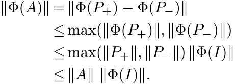
This proves the first inequality of the theorem. The second is obtained from this by using the Cartesian decomposition of T. ■
Exercise 2.5.4 shows that the factor 2 in the inequality (ii) of Theorem 2.6.3 is unavoidable in general. It can be dropped when k = 1:
2.6.4 Theorem
Let φ be a positive linear functional on an operator system ![]() . Then ||φ|| = φ(I).
. Then ||φ|| = φ(I).
Proof. Let ![]() and ||T|| ≤ 1. We want to show |φ(T)| ≤ φ(I). If φ(T) is the complex
number reiθ, we may multiply T by e−iθ, and thus assume φ(T) is real and positive.
So, if T = A+ iB in the Cartesian decomposition, then φ(T) = φ(A). Hence by part
(i) of Theorem 2.6.3 φ(T) ≤ φ(I)||A|| ≤ φ(I)||T||. ■
and ||T|| ≤ 1. We want to show |φ(T)| ≤ φ(I). If φ(T) is the complex
number reiθ, we may multiply T by e−iθ, and thus assume φ(T) is real and positive.
So, if T = A+ iB in the Cartesian decomposition, then φ(T) = φ(A). Hence by part
(i) of Theorem 2.6.3 φ(T) ≤ φ(I)||A|| ≤ φ(I)||T||. ■
The converse is also true.
2.6.5 Theorem
Let φ be a linear functional on ![]() such that ||φ|| = φ(I). Then φ is positive.
such that ||φ|| = φ(I). Then φ is positive.
Proof. Assume, without loss of generality, that φ(I) = 1. Let A be a positive element
of ![]() and let σ(A) be its spectrum. Let a = min σ(A) and b = max σ(A). We will show
that the point φ(A) lies in the interval [a, b]. If this is not the case, then there
exists a disk D = {z : |z − z0| ≤ r} such that φ(A) is outside D but D contains [a,
b], and hence also σ(A). From the latter condition it follows that σ(A−z0I) is contained
in the disk {z : |z| ≤ r} , and hence ||A−z0I|| ≤ r. Using the conditions ||φ|| =
φ(I) = 1, we get from this
and let σ(A) be its spectrum. Let a = min σ(A) and b = max σ(A). We will show
that the point φ(A) lies in the interval [a, b]. If this is not the case, then there
exists a disk D = {z : |z − z0| ≤ r} such that φ(A) is outside D but D contains [a,
b], and hence also σ(A). From the latter condition it follows that σ(A−z0I) is contained
in the disk {z : |z| ≤ r} , and hence ||A−z0I|| ≤ r. Using the conditions ||φ|| =
φ(I) = 1, we get from this
But then φ(A) could not have been outside D.
This shows that φ(A) is a nonnegative number, and the theorem is proved. ■
2.6.6 Theorem (The Krein Extension Theorem)
Let ![]() be an operator system in
be an operator system in ![]() . Then every positive linear functional on
. Then every positive linear functional on ![]() can be
extended to a positive linear functional on
can be
extended to a positive linear functional on ![]() .
.
Proof. Let φ be a positive linear functional on ![]() . By Theorem 2.6.4, ||φ|| = φ(I).
By the Hahn-Banach Theorem, φ can be extended to a linear functional
. By Theorem 2.6.4, ||φ|| = φ(I).
By the Hahn-Banach Theorem, φ can be extended to a linear functional ![]() on
on ![]() with
with ![]() .
But then
.
But then ![]() is positive by Theorem 2.6.5 (or by Exercise 2.5.1). ■
is positive by Theorem 2.6.5 (or by Exercise 2.5.1). ■
Finally we have the following theorem that proves the assertion made at the end of the discussion of Question 1 in Section 2.5.
2.6.7 Theorem
Let ![]() be an operator system and let
be an operator system and let ![]() k be a unital linear map such that ||Φ|| = 1.
Then Φ is positive.
k be a unital linear map such that ||Φ|| = 1.
Then Φ is positive.
Proof. For each unit vector x in ![]() , let
, let
This is a unital linear functional on ![]() . Since |φx(A)| ≤ ||Φ(A)|| ≤ ||A||, we have
||φx|| = 1. So, by Theorem 2.6.5, φx is positive. In other words, if A is positive,
then for every unit vector x
. Since |φx(A)| ≤ ||Φ(A)|| ≤ ||A||, we have
||φx|| = 1. So, by Theorem 2.6.5, φx is positive. In other words, if A is positive,
then for every unit vector x
But that means Φ is positive. ■
2.7 SUPPLEMENTARY RESULTS AND EXERCISES
Some of the theorems in Section 2.3 are extended in various directions in the following propositions.
2.7.1 Proposition
Let Φ be a positive unital linear map on ![]() and let A be a positive matrix. Then
and let A be a positive matrix. Then
Proof. Let 0 < r < 1. Using the integral representation (1.39) we have
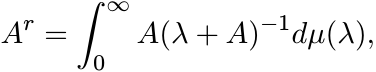
where µ is a positive measure on (0, ∞). So it suffices to show that
for all λ > 0. We have the identity
Apply Φ to both sides and use Theorem 2.3.6 to get
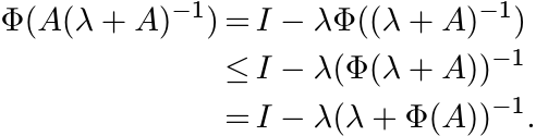
The identity stated above shows that the last expression is equal to Φ(A)(λ + Φ(A))−1. ■
2.7.2 Exercise
Let Φ be a positive unital linear map on ![]() and let A be a positive matrix. Show that
and let A be a positive matrix. Show that
if 1 ≤ r ≤ 2. If A is strictly positive, then this is true also when −1 ≤ r ≤ 0. [Hint: Use integral representations of Ar as in Theorem 1.5.8, Exercise 1.5.10, and the inequalities (2.5) and (2.7).]
2.7.3 Proposition
Let Φ be a strictly positive linear map on Mn. Then
whenever H is Hermitian and A > 0.
Proof. Let
Then Ψ is positive and unital. By Kadison’s inequality we have Ψ(Y 2) ≥ Ψ(Y )2 for every Hermitian Y . Choose Y = A−1/2HA−1/2 to get

Use (2.21) now to get (2.20). ■
2.7.4 Exercise
Construct an example to show that a more general version of (2.20)
where X is arbitrary and A positive, is not always true.
2.7.5 Proposition
Let Φ be a strictly positive linear map on ![]() and let A > O. Then
and let A > O. Then
Proof. Let Ψ be the linear map defined by (2.21). By the Russo-Dye theorem
Let A ≥ X∗A−1X and put Y = A−1/2XA−1/2. Then Y ∗Y = A−1/2 X∗A−1 XA−1/2 ≤ I. Hence Ψ(A−1/2X∗A−1/2)Ψ(A−1/2XA−1/2) ≤ I. Use (2.21) again to get (2.22). ■
In classical probability the quantity
is called the variance of the real function f. In analogy we consider
where A is Hermitian and Φ a positive unital linear map on ![]() . Kadison’s inequality
says var(A) ≥ O. The following proposition gives an upper bound for var(A).
. Kadison’s inequality
says var(A) ≥ O. The following proposition gives an upper bound for var(A).
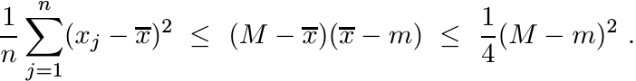
2.7.6 Proposition
Let Φ be a positive unital linear map and let A be a Hermitian operator with mI ≤ A ≤ MI. Then
 (2.25)
Proof. The matrices MI − A and A− mI are positive and commute with each other. So, (MI − A)(A − mI) ≥ O; i.e.,
Apply Φ to both sides and then subtract Φ(A)2 from both sides. This gives the first
inequality in (2.25). To prove the second inequality note that if m ≤ x ≤ M, then
![]() . ■
. ■
2.7.7 Exercise
Let ![]() . We say x ≥ 0 if all its coordinates xj are nonnegative. Let e = (1, . . . ,
1).
. We say x ≥ 0 if all its coordinates xj are nonnegative. Let e = (1, . . . ,
1).
A matrix S is called stochastic if sij ≥ 0 for all i, j, and ![]() for all i. Show that
S is stochastic if and only if
for all i. Show that
S is stochastic if and only if
and
The property (2.26) can be described by saying that the linear map defined by S on
![]() is positive, and (2.27) by saying that S is unital.
is positive, and (2.27) by saying that S is unital.
If x is a real vector, let ![]() . Show that if S is a stochastic matrix and m ≤ xj ≤ M,
then
. Show that if S is a stochastic matrix and m ≤ xj ≤ M,
then
 (2.28)
A special case of this is obtained by choosing ![]() for all i, j. If
for all i, j. If ![]() , this gives
, this gives
 (2.29)
An inequality complementary to (2.7) is given by the following proposition.
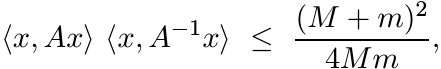
2.7.8 Proposition
Let Φ be strictly positive and unital. Let 0 < m < M. Then for every strictly positive matrix A with mI ≤ A ≤ MI, we have
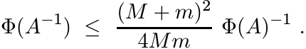 (2.30)
Proof. The matrices A − mI and MA−1 − I are positive and commute with each other. So, O ≤ (A − mI)(MA−1 − I). This gives
and hence
Now, if c and x are real numbers, then (c − 2x)2 ≥ 0 and therefore, for positive
x we have ![]() . So, we get
. So, we get
A very special corollary of this is the inequality
 (2.31)
for every unit vector x. This is called the Kantorovich inequality.
2.7.9 Exercise
Let f be a convex function on an interval [m, M] and let L be the linear interpolant

Show that if Φ is a unital positive linear map, then for every Hermitian matrix A whose spectrum is contained in [m, M], we have
Use this to obtain Propositions 2.7.6 and 2.7.8.
The space ![]() has a natural inner product defined as
has a natural inner product defined as
If Φ is a linear map on ![]() , we define its adjoint Φ∗ as the linear map that satisfies
the condition
, we define its adjoint Φ∗ as the linear map that satisfies
the condition
2.7.10 Exercise
The linear map Φ is positive if and only if Φ∗ is positive. Φ is unital if and only if Φ∗ is trace preserving; i.e., tr Φ∗(A) = tr A for all A.
We say Φ is a doubly stochastic map on ![]() if it is positive,unital, and trace preserving
(i.e., both Φ and Φ∗ are positive and unital).
if it is positive,unital, and trace preserving
(i.e., both Φ and Φ∗ are positive and unital).
2.7.11 Exercise
(i) Let Φ be the linear map on Mn defined as Φ(A) = X∗AX. Show that Φ∗(A) = XAX∗.
(ii) For any A, let SA(X) = A◦ X be the Schur product map. Show that (SA)∗ = SA∗.
(iii) Every pinching is a doubly stochastic map.
(iv) Let LA(X) = A∗X + XA be the Lyapunov operator, where A is a matrix with its spectrum in the open right half plane. Show that (L− A 1)∗ = (LA∗ )−1.
A norm ||| · ||| on Mn is said to be unitarily invariant if |||UAV ||| = |||A||| for all A and unitary U, V . It is convenient to make a normalisation so that |||A||| = 1 whenever A is a rank-one orthogonal projection.
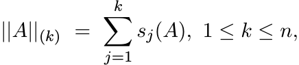
Special examples of such norms are the Ky Fan norms
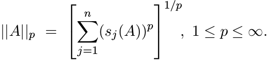
and the Schatten p-norms
Note that the operator norm, in this notation, is
and the trace norm is the norm
The norm ||A||2 is also called the Hilbert-Schmidt norm.
The following facts are well known:
If ||A||(k) ≤ ||B||(k) for 1 ≤ k ≤ n, then |||A||| ≤ |||B||| for all unitarily invariant norms. This is called the Fan dominance theorem. (See MA, p. 93.)
For any three matrices A, B, C we have
If Φ is a linear map on ![]() and ||| · ||| any unitarily invariant norm, then we use
the notation |||Φ||| for
and ||| · ||| any unitarily invariant norm, then we use
the notation |||Φ||| for
 (2.36)
In the same way,
etc.
The norm ||A||1 is the dual of the norm ||A|| on Mn. Hence
2.7.12 Exercise
Let ||| · ||| be any unitarily invariant norm on Mn.
(i) Use the relations (2.34) and the Fan dominance theorem to show that if ||Φ|| ≤ 1 and ||Φ∗|| ≤ 1, then |||Φ||| ≤ 1.
(ii) If Φ is a doubly stochastic map, then |||Φ||| ≤ 1.
(iii) If A ≥ O, then |||A ◦ X||| ≤ max aii|||X||| for all X.
(iv)
Let LA be the Lyapunov operator associated with a positively stable matrix A. We
know that ![]() . Show that in the special case when A is normal we have
. Show that in the special case when A is normal we have ![]() = [2 min Re λi]−1,
where λi are the eigenvalues of A.
= [2 min Re λi]−1,
where λi are the eigenvalues of A.
2.7.13 Exercise
Let A and B be Hermitian matrices. Suppose A = Φ(B) for some doubly stochastic map
Φ on Mn. Show that A is a convex combination of unitary conjugates of B; i.e., there
exist unitary matrices U1, . . . , Uk and positive numbers p1, . . . , pk with ![]() such
that
such
that
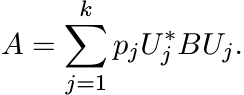
[Hints: There exist diagonal matrices D1 and D2, and unitary matrices W and V such
that A = W∗D1W and B = V D2V ∗. Use this to show that D1 = Ψ(D2) where Ψ is a doubly
stochastic map. By Birkhoff’s theorem there exist permutation matrices S1, . . .
, Sk and positive numbers p1, . . . , pk with ![]() such that
such that
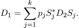
Choose Uj = V SjW. (Note that the matrices Uj and the numbers pj depend on Φ, A and B.)]
Let ![]() be the set of all n × n Hermitian matrices. This is a real vector space. Let
I be an open interval and let C1(I) be the space of continuously differentiable real
functions on I. Let
be the set of all n × n Hermitian matrices. This is a real vector space. Let
I be an open interval and let C1(I) be the space of continuously differentiable real
functions on I. Let ![]() be the set of all Hermitian matrices whose eigenvalues belong
to I. This is an open subset of
be the set of all Hermitian matrices whose eigenvalues belong
to I. This is an open subset of ![]() . Every function f in C1(I) induces a map
. Every function f in C1(I) induces a map ![]() from
from ![]() into
into ![]() . This induced map is differentiable and its derivative is given by an interesting
formula known as the Daleckii-Krein formula.
. This induced map is differentiable and its derivative is given by an interesting
formula known as the Daleckii-Krein formula.
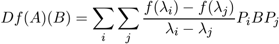
For each ![]() the derivative Df(A) at A is a linear map from
the derivative Df(A) at A is a linear map from ![]() into itself. If
into itself. If ![]() is the
spectral decomposition of A, then the formula is
is the
spectral decomposition of A, then the formula is
 (2.38)
for every ![]() . For i = j, the quotient in (2.38) is to be interpreted as f′(λi).
. For i = j, the quotient in (2.38) is to be interpreted as f′(λi).
This formula can be expressed in another way. Let f[1] be the function on I × I defined as
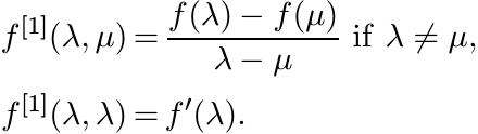
This is called the first divided difference of f. For ![]() , let f[1](A) be the n × n
matrix
, let f[1](A) be the n × n
matrix
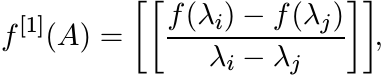 (2.39)
where λ1, . . . , λn are the eigenvalues of A. The formula (2.38) says
where ◦ denotes the Schur product taken in a basis in which A is diagonal. A proof of this is given in Section 5.3.
Suppose a real function f on an interval I has the following property: if A and
B are two elements of ![]() and A ≥ B, then f(A) ≥ f(B). We say that such a function f
is matrix monotone of order n on I. If f is matrix monotone of order n for all n
= 1, 2, . . . , then we say f is operator monotone.
and A ≥ B, then f(A) ≥ f(B). We say that such a function f
is matrix monotone of order n on I. If f is matrix monotone of order n for all n
= 1, 2, . . . , then we say f is operator monotone.
Matrix convexity of order n and operator convexity can be defined in a similar way. In Chapter 1 we have seen that the function f(t) = t2 on the interval [0, ∞) is not matrix monotone of order 2, and the function f(t) = t3 is not matrix convex of order 2. We have seen also that the function f(t) = tr on the interval [0, ∞) is operator monotone for 0 ≤ r ≤ 1, and it is operator convex for 1 ≤ r ≤ 2 and for −1 ≤ r ≤ 0. More properties of operator monotone and convex functions are studied in Chapters 4 and 5.
It is not difficult to prove the following, using the formula (2.40).
2.7.14 Exercise
If a function f ∈ C1(I) is matrix monotone of order n, then for each ![]() , the matrix
f[1](A) defined in (2.39) is positive.
, the matrix
f[1](A) defined in (2.39) is positive.
The converse of this statement is also true. A proof of this is given in Section 5.3. At the moment we note the following interesting consequence of the positivity of f[1](A).
2.7.15 Exercise
Let f ∈ C1(I) and let f′ be the derivative of f. Show that if f is matrix monotone
of order n, then for each ![]()
By definition
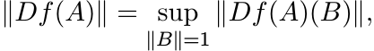 (2.42)
and
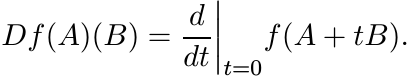
This expression is difficult to calculate for functions such as f(t) = tr, 0 < r < 1. The formula (2.41) gives an easy way to calculate its norm. Its effect is to reduce the supremum in (2.42) to the class of matrices B that commute with A.
2.8 NOTES AND REFERENCES
Since positivity is a useful and interesting property, it is natural to ask what linear transformations preserve it. The variety of interesting examples, and their interpretation as “expectation,” make positive linear maps especially interesting. Their characterization, however, has turned out to be slippery, and for various reasons the special class of completely positive linear maps has gained in importance.
Among the early major works on positive linear maps is the paper by E. Størmer, Positive linear maps of operator algebras, Acta Math., 110 (1963) 233–278. Research expository articles that explain several subtleties include E. Størmer, Positive linear maps of C∗-algebras, in Foundations of Quantum Mechanics and Ordered Linear Spaces, Lecture Notes in Physics, Vol. 29, Springer, 1974, pp.85–106, and M.-D. Choi, Positive linear maps, in Operator Algebras and Applications, Part 2, R. Kadison ed., American Math. Soc., 1982. Closer to our concerns are Chapter 2 of V. Paulsen, Completely Bounded Maps and Operator Algebras, Cambridge University Press, 2002, and sections of the two reports by T. Ando, Topics on Operator Inequalities, Sapporo, 1978 and Operator-Theoretic Methods for Matrix Inequalities, Sapporo, 1998.
The inequality (2.5) was proved in the paper R. Kadison, A generalized Schwarz inequality and algebraic invariants for operator algebras, Ann. Math., 56 (1952) 494–503. This was generalized by C. Davis, A Schwarz inequality for convex operator functions, Proc. Am. Math. Soc., 8 (1957) 42–44, and by M.-D. Choi, A Schwarz inequality for positive linear maps on C∗-algebras, Illinois J. Math., 18 (1974) 565–574. The generalizations say that if Φ is a positive unital linear map and f is an operator convex function, then we have a Jensen-type inequality
 (2.43)
The inequality (2.7) and the result of Exercise 2.7.2 are special cases of this. Using the integral representation of an operator convex function given in Problem V.5.5 of MA, one can prove the general inequality by the same argument as used in Exercise 2.7.2. The inequality (2.43) characterises operator convex functions, as was noted by C. Davis, Notions generalizing convexity for functions defined on spaces of matrices, in Proc. Symposia Pure Math., Vol. VII, Convexity, American Math. Soc., 1963.
In our proof of Theorem 2.3.7 we used the fact that any contraction is an average of two unitaries. The infinite-dimensional analogue says that the unit ball of a C∗-algebra is the closed convex hull of the unitary elements. (Unitaries, however, do not constitute the full set of extreme points of the unit ball. See P. R. Halmos, A Hilbert Space Problem Book, Second Edition, Springer, 1982.) This theorem about the closed convex hull is also called the Russo-Dye theorem and was proved in B. Russo and H. A. Dye, A note on unitary operators in C∗-algebras, Duke Math. J., 33 (1966) 413–416.
Applications given in Section 2.4 make effective use of Theorem 2.3.7 in calculating norms of complicated operators. Our discussion of the Lyapunov equation follows the one in R. Bhatia and L. Elsner, Positive linear maps and the Lyapunov equation, Oper. Theory: Adv. Appl., 130 (2001) 107–120. As pointed out in this paper, the use of positivity leads to much more economical proofs than those found earlier by engineers. The equality (2.15) was first proved by R. Bhatia and S. Friedland, Variation of Grassman powers and spectra, Linear Algebra Appl., 40 (1981) 1–18. The alternate proof using positivity is due to V. S. Sunder, A noncommutative analogue of |DXk| = |kXk−1|, ibid., 44 (1982) 87-95. The analogue of the formula (2.15) when the antisymmetric tensor product is replaced by the symmetric one was worked out in R. Bhatia, Variation of symmetric tensor powers and permanents, ibid., 62 (1984) 269–276. The harder problem embracing all symmetry classes of tensors was solved in R. Bhatia and J. A. Dias da Silva, Variation of induced linear operators, ibid., 341 (2002) 391–402.
Because of our interest in certain kinds of matrix problems involving calculation
or estimation of norms we have based our discussion in Section 2.5 on the relation
(2.16). There are far more compelling reasons to introduce operator systems. There
is a rapidly developing and increasingly important theory of operator spaces (closed
linear subspaces of C∗-algebras) and operator systems. See the book by V. Paulsen
cited earlier, E. G. Effros and Z.-J. Ruan, Operator Spaces, Oxford University Press,
2000, and G. Pisier, Introduction to Operator Space Theory, Cambridge University
Press, 2003. This is being called the noncommutative or quantized version of Banach
space theory. One of the corollaries of the Hahn-Banach theorem is that every separable
Banach space is isometrically isomorphic to a subspace of l∞; and every Banach space
is isometrically isomorphic to a subspace of l∞(X) for some set X. In the quantized
version the commutative space l∞ is replaced by the noncommutative space ![]() where
where ![]() is a Hilbert space. Of course, it is not adequate functional analysis to study just
the space l∞ and its subspaces. Likewise subspaces of
is a Hilbert space. Of course, it is not adequate functional analysis to study just
the space l∞ and its subspaces. Likewise subspaces of ![]() are called concrete operator
spaces, and then subsumed in a theory of abstract operator spaces.
are called concrete operator
spaces, and then subsumed in a theory of abstract operator spaces.
Our discussion in Section 2.6 borrows much from V. Paulsen’s book. Some of our proofs are simpler because we are in finite dimensions.
Propositions 2.7.3 and 2.7.5 are due to M.-D. Choi, Some assorted inequalities for positive linear maps on C∗-algebras, J. Operator Theory, 4 (1980) 271–285. Propositions 2.7.6 and 2.7.8 are taken from R. Bhatia and C. Davis, A better bound on the variance, Am. Math. Monthly, 107 (2000) 602–608. Inequalities (2.29), (2.31) and their generalizations are important in statistics, and have been proved by many authors, often without knowledge of previous work. See the article S. W. Drury, S. Liu, C.-Y. Lu, S. Puntanen, and G. P. H. Styan, Some comments on several matrix inequalities with applications to canonical correlations: historical background and recent developments, Sankhyā, Series A, 64 (2002) 453–507.
The Daleckii-Krein formula was presented in Ju. L. Daleckii and S. G. Krein, Formulas of differentiation according to a parameter of functions of Hermitian operators, Dokl. Akad. Nauk SSSR, 76 (1951) 13–16. Infinite dimensional analogues in which the double sum in (2.38) is replaced by a double integral were proved by M. Sh. Birman and M. Z. Solomyak, Double Stieltjes operator integrals (English translation), Topics in Mathematical Physics Vol. 1, Consultant Bureau, New York, 1967.
The formula (2.41) was noted in R. Bhatia, First and second order perturbation bounds
for the operator absolute value, Linear Algebra Appl., 208/209 (1994) 367–376. It
was observed there that this equality of norms holds for several other functions
that are not operator monotone. If A is positive and f(A) = Ar, then the equality
(2.41) is true for all real numbers r other than those in ![]() . This, somewhat mysterious,
result was proved in two papers: R. Bhatia and K. B. Sinha, Variation of real powers
of positive operators, Indiana Univ. Math. J., 43 (1994) 913–925, and R. Bhatia and
J. A. R. Holbrook, Fréchet derivatives of the power function, ibid., 49(2000) 1155–1173.
Similar equalities involving higher-order derivatives have been proved in R. Bhatia,
D. Singh, and K. B. Sinha, Differentiation of operator functions and perturbation
bounds, Commun. Math. Phys., 191 (1998) 603–611.
. This, somewhat mysterious,
result was proved in two papers: R. Bhatia and K. B. Sinha, Variation of real powers
of positive operators, Indiana Univ. Math. J., 43 (1994) 913–925, and R. Bhatia and
J. A. R. Holbrook, Fréchet derivatives of the power function, ibid., 49(2000) 1155–1173.
Similar equalities involving higher-order derivatives have been proved in R. Bhatia,
D. Singh, and K. B. Sinha, Differentiation of operator functions and perturbation
bounds, Commun. Math. Phys., 191 (1998) 603–611.