
Chapter Four
Matrix Means
Let a and b be positive numbers. Their arithmetic, geometric, and harmonic means are the familiar objects
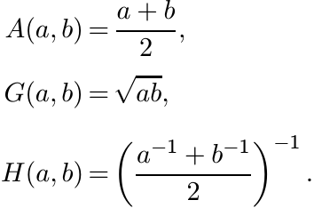
These have several properties that any object that is called a mean M(a, b) should have. Some of these properties are
(i) M(a, b) > 0,
(ii) If a ≤ b, then a ≤ M(a, b) ≤ b,
(iii) M(a, b) = M(b, a) (symmetry),
(iv) M(a, b) is monotone increasing in a, b,
(v) M(αa, αb) = αM(a, b) for all positive numbers a, b, and α,
(vi) M(a, b) is continuous in a, b.
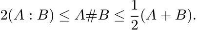
The three of the most familiar means listed at the beginning satisfy these conditions. We have the inequality
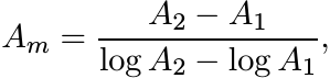
Among other means of a, b is the logarithmic mean defined as
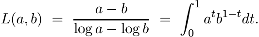 (4.2)
(4.2)This has the properties (i)–(vi) listed above. Further
This is a refinement of the arithmetic-geometric mean inequality—the second part of (4.1). See Exercise 4.5.5 and Lemma 5.4.5.
Averaging operations are of interest in the context of matrices as well, and various notions of means of positive definite matrices A and B have been studied. A mean M(A, B) should have properties akin to (i)–(vi) above. The order “≤” now is the natural order X ≤ Y on Hermitian matrices. It is obvious what the analogues of properties (i)–(vi) are for the case of positive definite matrices. Property (v) has another interpretation: for positive numbers a, b and any nonzero complex number x
It is thus natural to expect any mean M(A, B) to satisfy the condition
for all A, B > O and all nonsingular X. This condition is called congruence invariance and if the equality (v′) is true, we say that M is invariant under congruence. Restricting X to scalar matrices we see that
for all positive numbers α.
So we say that a matrix mean is a binary operation ![]() M(A, B) on the set of positive
definite matrices that satisfies (the matrix versions of ) the conditions (i)–(vi),
the condition (v) being replaced by (v′).
M(A, B) on the set of positive
definite matrices that satisfies (the matrix versions of ) the conditions (i)–(vi),
the condition (v) being replaced by (v′).
What are good examples of such means? The arithmetic mean presents no difficulties.
It is obvious that ![]() has all the six properties listed above. The harmonic mean of
A and B should be the matrix
has all the six properties listed above. The harmonic mean of
A and B should be the matrix ![]() . Now some of the properties (i)–(vi) are obvious, others
are not. It is not clear what object should be called the geometric mean in this
case. The product A1/2B1/2 is not Hermitian, let alone positive, unless A and B commute.
. Now some of the properties (i)–(vi) are obvious, others
are not. It is not clear what object should be called the geometric mean in this
case. The product A1/2B1/2 is not Hermitian, let alone positive, unless A and B commute.
In this chapter we define a geometric mean of positive matrices and study its properties along with those of the arithmetic and the harmonic mean. We use these ideas to prove some theorems on operator monotonicity and convexity. These theorems are then used to derive important properties of the quantum entropy. A positive matrix in this chapter is assumed to be strictly positive. Extensions of some of the considerations to positive semidefinite matrices are briefly indicated.
4.1 THE HARMONIC MEAN AND THE GEOMETRIC MEAN
The parallel sum of two positive matrices A, B is defined as the matrix
This definition could be extended to positive semidefinite matrices A, B by a limit from above:
 (4.5)
(4.5)
This operation was studied by Anderson and Duffin in connection with electric networks.
(If two wires with resistances r1 and r2 are connected in parallel, then their total
resistance r according to one of Kirchhoff ’s laws is given by ![]() .)
.)
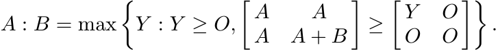
The harmonic mean of A, B is the matrix 2(A : B). To save on symbols we will not introduce a separate notation for it. Note that
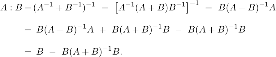 (4.6)
(4.6)By symmetry
Thus A : B is the Schur complement of A + B in either of the block matrices
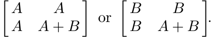
Several properties of A : B can be derived from this.
4.1.1 Theorem
For any two positive matrices A, B we have
(i) A : B ≤ A, A : B ≤ B.
(ii) A : B is monotonically increasing and jointly concave in the arguments A, B.
(iii)
 (4.8)
(4.8)Proof.
(i) The subtracted terms in (4.6) and (4.7) are positive.
(ii) See Corollary 1.5.3.
(iii) See Corollary 1.5.5. ■
4.1.2 Proposition
If A ≤ B, then A ≤ 2(A : B) ≤ B.
Proof.
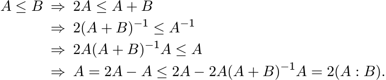
A similar argument shows 2(A : B) ≤ B. ■
Thus the harmonic mean satisfies properties (i)–(v) listed at the beginning of the chapter. (Notice one difference: for positive numbers a, b either a ≤ b or b ≤ a; this is not true for positive matrices A, B.)
How about the geometric mean of A, B? If A, B commute, then their geometric mean
can be defined as A1/2B1/2. But this is the trivial case. In all other cases this
matrix is not even Hermitian. The matrix ![]() is Hermitian but not always positive. Positivity
is restored if we consider
is Hermitian but not always positive. Positivity
is restored if we consider
It turns out that this is not monotone in A, B. (Exercise: construct a 2 × 2 example to show this.) One might try other candidates; e.g., e(log A+log B)/2, that reduce to a1/2b1/2 for positive numbers. This particular one is not monotone.
Here the property (v′)—congruence invariance—that we expect a mean to have is helpful. We noted in Exercise 1.6.1 that any two positive matrices are simultaneously congruent to diagonal matrices. The geometric mean of two positive diagonal matrices A and B, naturally, is A1/2B1/2.
Let us introduce a notation and state a few elementary facts that will be helpful
in the ensuing discussion. Let GL(n) be the group consisting of n × n invertible
matrices. Each element X of GL(n) gives a congruence transformation on ![]() . We write
this as
. We write
this as
The collection {ΓX : X ∈ GL(n)} is a group of transformations on Mn. We have ΓXΓY
= ΓY X and ![]() . This group preserves the set of positive matrices. Given a pair of matrices
A, B we write ΓX(A, B) for (ΓX(A), ΓX (B)) .
. This group preserves the set of positive matrices. Given a pair of matrices
A, B we write ΓX(A, B) for (ΓX(A), ΓX (B)) .
Let A, B be positive matrices. Then
We can find a unitary matrix U such that ![]() , a diagonal matrix. So
, a diagonal matrix. So
The geometric mean of the matrices I and D is
So, if the geometric mean of two positive matrices A and B is required to satisfy the property (v′), then it has to be the matrix
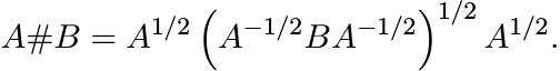 (4.10)
If A and B commute, then A#B = A1/2B1/2. The expression (4.10) does not appear to be symmetric in A and B. However, it is. This is seen readily from another description of A#B. By Exercise 1.2.13 the matrix in (4.10) is the unique positive solution of the equation
If we take inverses of both sides, then this equation is transformed to XB−1X = A. This shows that
Using Theorem 1.3.3 and the relation
that we have just proved, we see that
 (4.13)
On the other hand if X is any Hermitian matrix such that
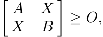 (4.14)
then again by Theorem 1.3.3, we have A ≥ XB−1X. Hence
Taking square roots and then applying the congruence ΓB1/2 , we get from this
In other words A#B ≥ X for any Hermitian matrix X that satisfies the inequality (4.14).
The following theorem is a summary of our discussion so far.
4.1.3 Theorem
Let A and B be two positive matrices. Let
Then
(i) A#B = B#A,
(ii) A#B is the unique positive solution of the equation XA−1X = B,
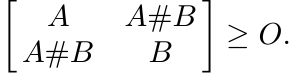
(iii) A#B has an extremal property:
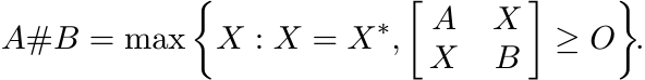 (4.15)
The properties (i)–(vi) listed at the beginning of the chapter can be verified for A#B using one of the three characterizations given in Theorem 4.1.3. Thus, for example, the symmetry (4.12) is apparent from (4.15) as well. Monotonicity in the variable B is apparent from (4.10) and Proposition 1.2.9; and then by symmetry we have monotonicity in A. This is plain from (4.15) too. From (4.15) we see that A#B is jointly concave in A and B.
Since congruence operations preserve order, the inequality (4.1) is readily carried over to operators. We have
 (4.16)
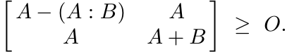
It is easy to see either from (4.10) or from Theorem 4.1.3 (ii) that
4.1.4 Exercise
Use the characterization (4.15) and the symmetry (4.12) to give another proof of the second inequality in (4.16). Use (4.15) and (4.17) to give another proof of the first inequality in (4.16).
If A or B is not strictly positive, we can define their geometric mean by a limiting procedure, as we did in (4.5) for the parallel sum.
The next theorem describes the effect of positive linear maps on these means.
4.1.5 Theorem
Let Φ be any positive linear map on ![]() . Then for all positive matrices A, B
. Then for all positive matrices A, B
(i) Φ(A : B) ≤ Φ(A) : Φ(B);
(ii) Φ(A#B) ≤ Φ(A)#Φ(B).
Proof. (i) By the extremal characterization (4.8)
By Exercise 3.2.2 (ii), we get from this

Again, by (4.8) this means Φ(A : B) ≤ Φ(A) : Φ(B).
The proof of (ii) is similar to this. Use the extremal characterization (4.15) for A#B, and Exercise 3.2.2 (ii). ■
For the special map ΓX(A) = X∗AX, where X is any invertible matrix the two sides of (i) and (ii) in Theorem 4.1.5 are equal.This need not be the case if X is not invertible.
4.1.6 Exercise
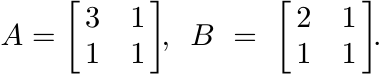
Let A, B, and X be the 2 × 2 matrices
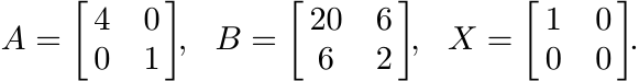
Show that

So, if Φ(A) = X∗AX, then in this example we have
The inequality (4.13) and Proposition 1.3.2 imply that there exists a contraction K such that A#B = A1/2KB1/2. More is true as the next Exercise and Proposition show.
4.1.7 Exercise
Let U = (A−1/2BA−1/2)1/2A1/2B−1/2. Show that U∗U = UU∗ = I. Thus we can write
where U is unitary.
It is an interesting fact that this property characterizes the geometric mean:
4.1.8 Proposition
Let A, B be positive matrices and suppose U is a unitary matrix such that A1/2UB1/2 is positive. Then A1/2UB1/2 = A#B.
Proof. Let G = A1/2UB1/2. Then

We have another congruence

(See the proof of Theorem 1.3.3.) Note that the matrix ![]() has rank n. Since congruence
preserves rank we must have A = GB−1G. But then, by Theorem 4.1.3 (ii), G = A#B.
■
has rank n. Since congruence
preserves rank we must have A = GB−1G. But then, by Theorem 4.1.3 (ii), G = A#B.
■
Two more ways of expressing the geometric mean are given in the following propositions. We use here the fact that if X is a matrix with positive eigenvalues, then it has a unique square root Y with positive eigenvalues. A proof is given in Exercise 4.5.2.
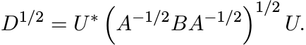
4.1.9 Proposition
Let A, B be positive matrices and let ![]() be the the square root of A−1B that has positive
eigenvalues. Then
be the the square root of A−1B that has positive
eigenvalues. Then
Proof. We have the identity

Taking square roots, we get
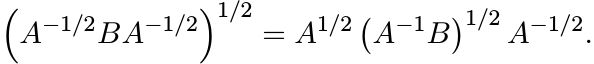
This, in turn, shows that

4.1.10 Exercise
Show that for positive matrices A, B we have
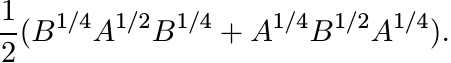
4.1.11 Proposition
Let A, B be positive matrices. Then
(The matrix inside the square brackets has positive eigenvalues and the square root chosen is the one with positive eigenvalues.)
Proof. Use the identity
to get
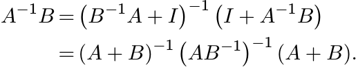
Taking square roots, we get
This gives
Using Proposition 4.1.9 and Exercise 4.1.10, we get from this
Premultiply both sides by (A + B)−,1 and then take square roots, to get
This proves the proposition. ■
On first sight, the three expressions in 4.1.9–4.1.11 do not seem to be positive matrices, nor do they seem to be symmetric in A, B.
The expression (4.10) and the ones given in Propositions 4.1.9 and 4.1.11 involve finding square roots of matrices, as should be expected in any definition of geometric mean. Calculating these square roots is not an easy task. For 2 × 2 matrices we have a formula that makes computation easier.
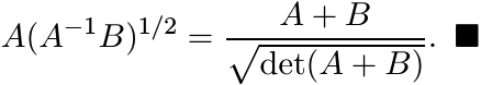
4.1.12 Proposition
Let A and B be 2 × 2 positive matrices each of which has determinant one. Then
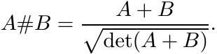
Proof. Use the formula given for A#B in Proposition 4.1.9. Let X = (A−1B)1/2. Then det X = 1 and so X has two positive eigenvalues λ and 1/λ. Further,
and hence tr ![]() . So, by the Cayley-Hamilton theorem
. So, by the Cayley-Hamilton theorem
Multiply on the left by A and rearrange terms to get
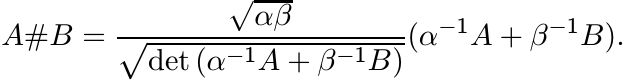
Exercise. Let A and B be 2×2 positive matrices and let det A = α2, det B = β2. Then
4.2 SOME MONOTONICITY AND CONVEXITY THEOREMS
In Section 5 of Chapter 1 and Section 7 of Chapter 2 we have discussed the notions of monotonicity, convexity and concavity of operator functions. Operator means give additional information as well as more insight into these notions. Some of the theorems in this section have been proved by different arguments in Chapter 1.
4.2.1 Theorem
If A ≥ B ≥ O, then Ar ≥ Br for all 0 ≤ r ≤ 1.
Proof. We know that the assertion is true for r = 0, 1. Suppose r1, r2 are two real numbers for which Ar1 ≥ Br1 and Ar2 ≥ Br2. Then, by monotonicity of the geometric mean, we have Ar1 #Ar2 ≥ Br1 #Br2. This is the same as saying A(r1+r2)/2 ≥ B(r1+r2)/2. Thus, the set of real numbers r for which Ar ≥ Br is a closed convex set. Since 0 and 1 belong to this set, so does the entire interval [0, 1]. ■
4.2.2 Exercise
We know that the function f(t) = t2 is not matrix monotone of order 2. Show that
the function f(t) = tr on ![]() is not matrix monotone of order 2 for any r > 1. [Hint:
Prove this first for r > 2.]
is not matrix monotone of order 2 for any r > 1. [Hint:
Prove this first for r > 2.]
It is known that a function f from ![]() into itself is operator monotone if and only
if it is operator concave. For the functions f(t) = tr, 0 ≤ r ≤ 1, operator concavity
is easily proved:
into itself is operator monotone if and only
if it is operator concave. For the functions f(t) = tr, 0 ≤ r ≤ 1, operator concavity
is easily proved:
4.2.3 Theorem
For 0 < r < 1, the map ![]() on positive matrices is concave.
on positive matrices is concave.
Proof. Use the representation
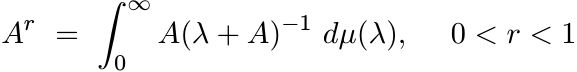 (4.18)
(see Theorem 1.5.8). The integrand
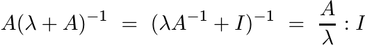
is concave in A by Theorem 4.1.1. Hence, so is the integral. (The integrand is also monotone in A. In Section 1.5 we used this argument to prove Theorem 4.2.1 and some other statements.) ■
4.2.4 Exercise
For 0 < r < 1, the map ![]() on positive matrices is monotone decreasing and convex.
[Use the facts that
on positive matrices is monotone decreasing and convex.
[Use the facts that ![]() is monotone and concave, and
is monotone and concave, and ![]() is monotone decreasing and convex.]
See Exercise 1.5.10 also.
is monotone decreasing and convex.]
See Exercise 1.5.10 also.
4.2.5 Exercise
The map ![]() log A on positive matrices is monotone and concave.
log A on positive matrices is monotone and concave.
[Hint: ![]() .]
.]
4.2.6 Exercise
The map ![]() −Alog A on positive matrices is concave.
−Alog A on positive matrices is concave.
[Hint: ![]() . Use Theorem 1.5.8.]
. Use Theorem 1.5.8.]
Some results on convexity of tensor product maps can be deduced easily using the harmonic mean. The following theorem was proved by Lieb. This formulation and proof are due to Ando.
4.2.7 Theorem
For 0 < r < 1, the map ![]() is jointly concave and monotone on pairs of positive
matrices A, B.
is jointly concave and monotone on pairs of positive
matrices A, B.
Proof. Note that ![]() . So, by the representation (4.18) we have
. So, by the representation (4.18) we have

The integrand can be written as
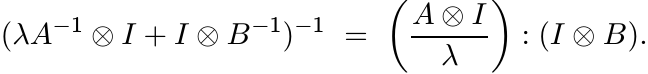
This is monotone and jointly concave in A, B. Hence, so is f (A, B). ■
4.2.8 Exercise
Let r1, r2 be positive numbers with r1 + r2 ≤ 1. Show that f(A, B) = ![]() is jointly
concave and monotone on pairs of positive matrices A, B. [Hint: Let r1 + r2 = r.
Then
is jointly
concave and monotone on pairs of positive matrices A, B. [Hint: Let r1 + r2 = r.
Then ![]() .]
.]
4.2.9 Exercise
Let r1, r2, . . . , rk be positive numbers with r1 + · · · + rk = 1. Then the product
![]() is jointly concave on k-tuples of positive matrices A1, . . . , Ak.
is jointly concave on k-tuples of positive matrices A1, . . . , Ak.
A special case of this says that for k = 1, 2, . . . , the map ![]()
![]() on positive matrices
is concave. This leads to the inequality
on positive matrices
is concave. This leads to the inequality
By restricting to symmetry classes of tensors one obtains inequalities for other induced operators. For example
For k = n, this reduces to the famous Minkowski determinant inequality
It is clear that many inequalities of this kind are included in the master inequality (4.19).
4.2.10 Exercise
For 0 ≤ r ≤ 1, the map ![]() is jointly convex on pairs of positive matrices A, B. [Hint:
is jointly convex on pairs of positive matrices A, B. [Hint:
![]()
![]() .]
.]
4.3 SOME INEQUALITIES FOR QUANTUM ENTROPY
Theorem 4.2.7 is equivalent to a theorem of Lieb on the concavity of one of the matrix functions arising in the study of entropy in quantum mechanics. We explain this and related results briefly.
Let (p1, . . . , pk) be a probability vector; i.e., pj ≥ 0 and ![]() . The function
. The function
called the entropy function, is of fundamental importance in information theory.
In quantum mechanics, the role analogous to that of (p1, . . . , pk) is played by a positive matrix A with tr A = 1. Such a matrix is called a density matrix. The entropy of A is defined as
The condition tr A = 1 is not essential for some of our theorems; and we will drop it some times.
It is easy to see that the function (4.22) is jointly concave in pj. An analogous result is true for the quantum mechanical entropy (4.23). In fact we have proved a much stronger result in Exercise 4.2.6. The proof of concavity of the scalar function (4.23) does not require the machinery of operator concave function.
4.3.1 Exercise
Let A be any Hermitian matrix and f any convex function on ![]() . Then for every unit
vector x
. Then for every unit
vector x
Use this to prove that S(A) is a concave function of A. [Hint: Choose an orthonormal
basis {ui} consisting of eigenvectors of ![]() . Show that for any convex function f
. Show that for any convex function f
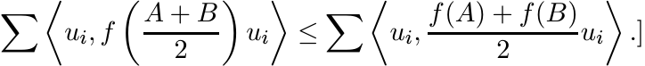
4.3.2 Proposition
Let f be a convex differentiable function on ![]() and let A, B be any two Hermitian matrices.
Then
and let A, B be any two Hermitian matrices.
Then
Proof. Let {ui} be an orthonormal basis whose elements are eigenvectors of B corresponding to eigenvalues βi. Then
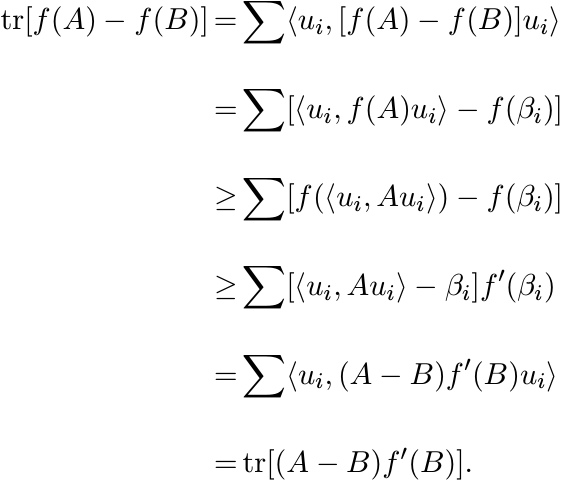
The first inequality in this chain follows from (4.24) and the second from the convexity of f. ■
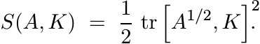
Other notions of entropy have been introduced in classical information theory and in quantum mechanics. One of them is called skew entropy or entropy of A relative to K, where A is positive and K Hermitian. This is defined as
 (4.26)
More generally we may consider for 0 < t < 1 the function
 (4.27)
Here [X, Y ] is the Lie bracket XY − Y X. Note that
The quantity (4.26) was introduced by Wigner and Yanase, (4.27) by Dyson. These are measures of the amount of noncommutativity of A with a fixed Hermitian operator K. The Wigner-Yanase-Dyson conjecture said St(A, K) is concave in A for each K. Note that tr (−K2A) is linear in A. So, from the expression (4.28) we see that the conjecture says that for each K, and for 0 < t < 1, the function tr KAtKA1−t is concave in A. A more general result was proved by Lieb in 1973.
4.3.3 Theorem (Lieb)
For any matrix X, and for 0 ≤ t ≤ 1, the function
is jointly concave on pairs of positive matrices A, B.
Proof. We will show that Theorems 4.2.7 and 4.3.3 are equivalent.
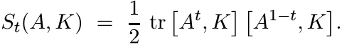
The tensor product ![]() and the space
and the space ![]() are isomorphic. The isomorphism φ acts as
are isomorphic. The isomorphism φ acts as ![]() . If
ei, 1 ≤ i ≤ n is the standard basis for
. If
ei, 1 ≤ i ≤ n is the standard basis for ![]() , and Eij the matrix units in
, and Eij the matrix units in ![]() , then
, then
From this one can see that
Thus φ is an isometric isomorphism between the Hilbert space ![]()
![]() and the Hilbert space
and the Hilbert space
![]() (the latter with the inner product
(the latter with the inner product ![]() ).
).
Let ![]() be the map induced by φ on operators; i.e.,
be the map induced by φ on operators; i.e., ![]() makes the diagram
makes the diagram
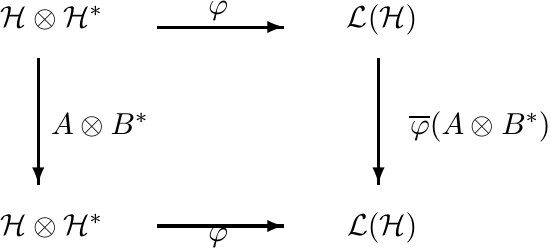
commute. It is easy to see that
So
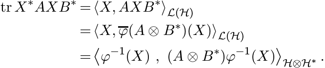
Thus for positive A, B, the concavity of tr X∗AtXB1−t is equivalent to the concavity
of ![]() . ■
. ■
Other useful theorems can be derived from Theorem 4.3.3. Here is an example. The
concept of relative entropy in classical information theory is defined as follows.
Let p, q be two probability distributions; i.e., p = (p1, . . . , pk), q = (q1, .
. . , qk), pj ≥ 0, qj ≥ 0, ![]() 1. Their relative entropy is defined as
1. Their relative entropy is defined as
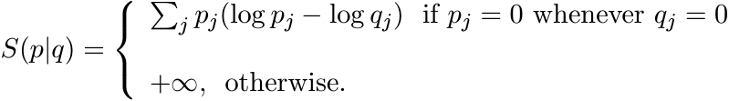
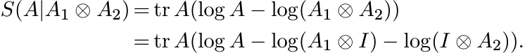
The relative entropy of density matrices A, B is defined as
4.3.4 Exercise (Klein’s Inequality)
For positive matrices A, B
[Hint: Use Proposition 4.3.2. with f(x) = x log x]. Thus, if A, B are density matrices, then
Note
(I is not a density matrix.) We have seen that S(A|I) is a convex function of A.
4.3.5 Theorem
The relative entropy S(A|B) is a jointly convex function of A and B.
Proof. For A positive and X arbitrary, let
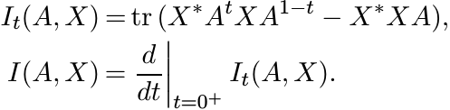
By Lieb’s theorem It(A, X) is a concave function of A. Hence, so is I(A, X). Note that
Now, given the positive matrices A, B let T, X be the 2 × 2 block matrices
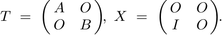
Then I(T, X) = −S(A|B). Since I(T, X) is concave, S(A|B) is convex. ■
The next few results describe the behaviour of the entropy function (4.23) with respect to tensor products. Here the condition tr A = 1 will be crucial for some of the statements.
4.3.6 Proposition
Let A, B be any two density matrices. Then
Proof. Let A, B have eigenvalues λ1, . . . , λn and µ1, . . . , µm, respectively.
Then ![]() , and
, and ![]() . The tensor product
. The tensor product ![]() has eigenvalues λiµj, 1 ≤ i ≤ n, 1 ≤ j ≤ m. So
has eigenvalues λiµj, 1 ≤ i ≤ n, 1 ≤ j ≤ m. So
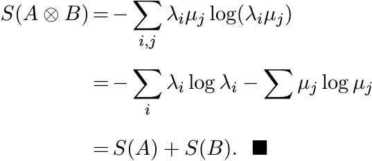
The equation (4.33) says that the entropy function S is additive with respect to tensor products.
Now let ![]() be two Hilbert spaces, and let
be two Hilbert spaces, and let ![]() . The operator A is called decomposable if
. The operator A is called decomposable if
![]() where A1, A2 are operators on
where A1, A2 are operators on ![]() . Not every operator on
. Not every operator on ![]() is decomposable. We associate
with every operator A on
is decomposable. We associate
with every operator A on ![]() two operators A1, A2 on
two operators A1, A2 on ![]() called the partial traces of A.
These are defined as follows.
called the partial traces of A.
These are defined as follows.
Let dim ![]() , dim H2 = m and let e1, . . . , em be an orthonormal basis in
, dim H2 = m and let e1, . . . , em be an orthonormal basis in ![]() . For
. For ![]() its
partial trace
its
partial trace ![]() is an operator on
is an operator on ![]() defined by the relation
defined by the relation
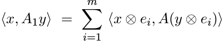 (4.34)
for all ![]() .
.
4.3.7 Exercise
The operator A1 above is well defined. (It is independent of the basis {ei} chosen
for ![]() .)
.)
The partial trace ![]() is defined in an analogous way.
is defined in an analogous way.
It is clear that if A is positive, then so are the partial traces A1, A2; and if
A is a density matrix, then so are A1, A2. Further, if ![]() A2 and A1, A2 are density
matrices, then
A2 and A1, A2 are density
matrices, then ![]() .
.
4.3.8 Exercise
Let A be an operator on ![]() with partial traces A1, A2. Then for every decomposable
operator B of the form
with partial traces A1, A2. Then for every decomposable
operator B of the form ![]() on
on ![]() we have
we have
The next proposition is called the subadditivity property of entropy.
4.3.9 Proposition
Let A be a density matrix in ![]() with partial traces A1, A2. Then
with partial traces A1, A2. Then
Proof. The matrix ![]() is a density matrix. So, by Exercise 4.3.4, the relative entropy
is a density matrix. So, by Exercise 4.3.4, the relative entropy
![]() is positive. By definition
is positive. By definition
By Exercise 4.3.8, this shows
 (4.37)
Since this quantity is positive, we have the inequality in (4.36). ■
There is another way of looking at the partial trace operation that is more transparent and makes several calculations easier:
4.3.10 Proposition
Let f1, . . . , fn and e1, . . . , em be orthonormal bases for ![]() and
and ![]() . Let A be an
operator on
. Let A be an
operator on ![]() and write its matrix in the basis
and write its matrix in the basis ![]() in the n × n partitioned form
in the n × n partitioned form
where Aij, 1 ≤ i, j ≤ n are m × m matrices. Then ![]() is the n × n matrix defined as
is the n × n matrix defined as
Proof. It is not difficult to derive this relation from (4.34). ■
4.3.11 Exercise
The map ![]() is the composition of three special kinds of maps described below.
is the composition of three special kinds of maps described below.
(i)
Let ω = e2πi/m and let U = diag(1, ω, . . . , ωm−1). Let W be the n × n block-diagonal
matrix ![]() (n copies). Let
(n copies). Let
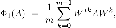 (4.40)
where A is as in (4.38). Show that
(See (3.28)).
(ii) Let V be the m × m permutation matrix defined as
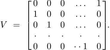
Let X be the n × n block-diagonal matrix ![]() (n copies). Let
(n copies). Let
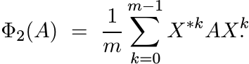 (4.42)
Show that
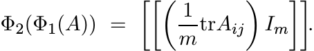 (4.43)
Thus the effect of Φ2 on the block matrix (4.41) is to replace each of the diagonal matrices Aij by the scalar matrix with the same trace as Aij.
(iii)
Let A be as in (4.38) and let ![]() be the (1,1) entry of Aij. Let
be the (1,1) entry of Aij. Let
 (4.44)
Note that the matrix ![]() is a principal n × n submatrix of A. We have then
is a principal n × n submatrix of A. We have then
(iv) Each of the maps Φ1, Φ2, Φ3 is completely positive; Φ1, Φ2, and Φ3Φ2Φ1 are trace preserving.
The next theorem says that taking partial traces of A, B reduces the relative entropy S(A|B).
4.3.12 Theorem
Let A, B be density matrices on ![]() . Then
. Then
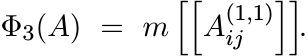
Proof. It is clear from the definition (4.29) that
for every unitary matrix U. Since S(A|B) is jointly convex in A, B by Theorem 4.3.5, it follows from the representations (4.40) and (4.42) that
Now note that Φ2Φ1(A) is a matrix of the form ![]() and Φ3 maps it to the n × n matrix
[[αij]]. Thus
and Φ3 maps it to the n × n matrix
[[αij]]. Thus
This proves the theorem. ■
4.3.13 Exercise
Let ![]() be any completely positive trace-preserving map. Use Stinespring’s theorem (Theorem
3.1.2) to show that
be any completely positive trace-preserving map. Use Stinespring’s theorem (Theorem
3.1.2) to show that
The inequality (4.46) is a special case of this.
Now we can state and prove the major result of this section: the strong subadditivity
of the entropy function S(A). This is a much deeper property than the subadditivity
property (4.36). It is convenient to adopt some notations. We have three Hilbert
spaces ![]()
![]() ; A123 stands for a density matrix on
; A123 stands for a density matrix on ![]() . A partial trace like
. A partial trace like ![]() is denoted
as A12, and so on for other indices. Likewise a partial trace
is denoted
as A12, and so on for other indices. Likewise a partial trace ![]() is denoted by A2.
is denoted by A2.
4.3.14 Theorem (Lieb-Ruskai)
Let A123 be any density matrix in ![]() . Then
. Then
Proof. By Theorem 4.3.12, taking the partial trace ![]() gives
gives
The equation (4.37) gives
and
Together, these three relations give (4.49). ■
4.4 FURUTA’S INEQUALITY
We have seen that the function f(A) = A2 is not order preserving on positive matrices; i.e., we may have A and B for which A ≥ B ≥ O but not A2 ≥ B2. Can some weaker form of monotonicity be retrieved for the square function? This question can have different meanings. For example, we can ask whether the condition A ≥ B ≥ O leads to an operator inequality implied by A2 ≥ B2. For positive matrices A and B consider the statements
(i) A2 ≥ B2;
(ii) BA2B ≥ B4;
(iii) (BA2B)1/2 ≥ B2.
Clearly (i) ![]() (ii)
(ii) ![]() (iii). Let A ≥ B. We know that the inequality (i) does not always
hold in this case. Nor does the weaker inequality (ii). A counterexample is provided
by
(iii). Let A ≥ B. We know that the inequality (i) does not always
hold in this case. Nor does the weaker inequality (ii). A counterexample is provided
by
The matrix ![]() has determinant −1.
has determinant −1.
It turns out that the inequality (iii) does follow from A ≥ B.
Note also that A2 ≥ B2 ![]() A4 ≥ AB2A
A4 ≥ AB2A ![]() A2 ≥ (AB2A)1/2. Once again, for A, B in the example
given above we do not have A4 ≥ AB2A. But we will see that A ≥ B always implies A2
≥ (AB2A)1/2.
A2 ≥ (AB2A)1/2. Once again, for A, B in the example
given above we do not have A4 ≥ AB2A. But we will see that A ≥ B always implies A2
≥ (AB2A)1/2.
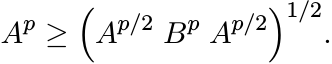
The most general result inspired by these considerations was proved by T. Furuta. To put it in perspective, consider the following statements:
(i) A ≥ B ≥ O;
(ii) Ap ≥ Bp, 0 ≤ p ≤ 1;
(iii) BrApBr ≥ Bp+2r, 0 ≤ p ≤ 1, r ≥ 0;
(iv) (BrApBr)1/q ≥ (Bp+2r)1/q, 0 ≤ p ≤ 1, r ≥ 0, q ≥ 1.
We know that (i) ![]() (ii)
(ii) ![]() (iii)
(iii) ![]() (iv). When p > 1, the implication (i)
(iv). When p > 1, the implication (i) ![]() (ii) breaks
down. Furuta’s inequality says that (iv) is still valid for all p but with some restriction
on q.
(ii) breaks
down. Furuta’s inequality says that (iv) is still valid for all p but with some restriction
on q.
4.4.1 Theorem (Furuta’s Inequality)
Let A ≥ B ≥ O. Then
for ![]() .
.
Proof. For 0 ≤ p ≤ 1, the inequality (4.50) is true even without the last restriction
on q. So assume p ≥ 1. If ![]() , then
, then ![]() . So, the inequality (4.50) holds for such q provided
it holds in the special case
. So, the inequality (4.50) holds for such q provided
it holds in the special case ![]() . Thus we need to prove
. Thus we need to prove
for p ≥ 1, r ≥ 0. We may assume that A, B are strictly positive. Let
be the polar decomposition. Then
Hence, for any q > 0
and, therefore (using (4.52) thrice) we get
 (4.53)
Now suppose 0 ≤ r ≤ 1/2. Then A2r ≥ B2r, and hence B−2r ≥ A−2r. Choose ![]() . Then
. Then ![]() .
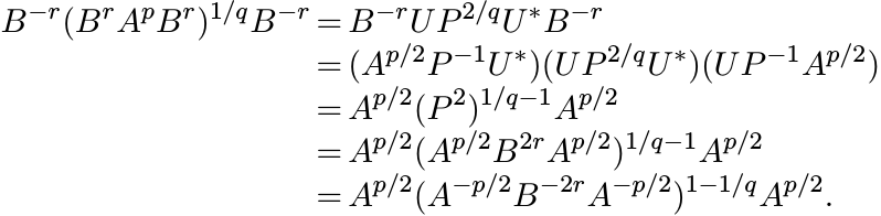
So, we get from (4.53)
.
So, we get from (4.53)
B−r(BrApBr)1/qB−r ≥ Ap/2(A−p/2A−2rA−p/2)(p−1)/(p+2r)Ap/2 = A.
Thus
We have thus proved the inequality (4.51) for r in the domain [0, 1/2]. This domain is extended by inductive steps as follows. Let
where r ∈ [0, 1/2] and q = (p + 2r)/(1 + 2r). We have proved that A1 ≥ B1. Let p1, r1 be any numbers with p1 ≥ 1, r1 ∈ [0, 1/2] and let q1 = (p1 + 2r1)/(1 + 2r1). Apply the inequality (4.54) to A1, B1, p1, r1, q1 to get
This is true, in particular, when p1 = q and r1 = 1/2. So we have
Substitute the values of A1, B1 from (4.55) to get from this
Put 2r + 1/2 = s, and note that with the choices just made
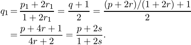
So, (4.57) can be written as
where s ∈ [1/2, 3/2]. Thus we have enlarged the domain of validity of the inequality (4.51) from r in [0, 1/2] to r in [0, 3/2]. The process can be repeated to see that the inequality is valid for all r ≥ 0. ■
4.4.2 Corollary
Let A, B, p, q, r be as in the Theorem. Then
Proof. Assume A, B are strictly positive. Since B−1 ≥ A−1 > O, (4.50) gives us
Taking inverse on both sides reverses this inequality and gives us (4.58). ■
4.4.3 Corollary
Let A ≥ B ≥ O, p ≥ 1, r ≥ 0. Then
4.4.4 Corollary
Let A ≥ B ≥ O. Then
These are the statements with which we began our discussion in this section. Another special consequence of Furuta’s inequality is the following.
4.4.5 Corollary
Let A ≥ B ≥ O. Then for 0 < p < ∞
Proof. Choose r = p/2 and q = 2 in (4.58) to get
This is equivalent to the inequality

Using the relation (4.17) we get (4.63). ■
For 0 ≤ p ≤ 1, the inequality (4.63) follows from Theorem 4.2.1. While the theorem does need this restriction on p, the inequality (4.63) exhibits a weaker monotonicity of the powers Ap for p > 1.
4.5 SUPPLEMENTARY RESULTS AND EXERCISES
The matrix equation
is called the Sylvester equation. If no eigenvalue of A is an eigenvalue of B, then for every Y this equation has a unique solution X. The following exercise outlines a proof of this.
4.5.1 Exercise
(i)
Let ![]() . This is a linear operator on
. This is a linear operator on ![]() . Each eigenvalue of A is an eigenvalue of
. Each eigenvalue of A is an eigenvalue of ![]() with
multiplicity n times as much. Likewise the eigenvalues of the operator
with
multiplicity n times as much. Likewise the eigenvalues of the operator ![]() are the eigenvalues
of B.
are the eigenvalues
of B.
(ii)
The operators ![]() and
and ![]() commute. So the spectrum of
commute. So the spectrum of ![]() is contained in the difference
is contained in the difference ![]() ,
where
,
where ![]() stands for the spectrum of
stands for the spectrum of ![]() .
.
(iii)
Thus if σ(A) and σ(B) are disjoint, then ![]() does not contain the point 0. Hence the
operator
does not contain the point 0. Hence the
operator ![]() is invertible. This is the same as saying that for each Y, there exists
a unique X satisfying the equation (4.64).
is invertible. This is the same as saying that for each Y, there exists
a unique X satisfying the equation (4.64).
The Lyapunov equation (1.14) is a special type of Sylvester equation.
There are various ways in which functions of an arbitrary matrix may be defined. One standard approach via the Jordan canonical form tells us how to explicitly write down a formula for f(A) for every function that is n − 1 times differentiable on an open set containing σ(A). Using this one can see that if A is a matrix whose spectrum is in (0, ∞), then it has a square root whose spectrum is also in (0, ∞). Another standard approach using power series expansions is equally useful.
4.5.2 Exercise
Let ![]() and
and ![]() . Then
. Then
Suppose all eigenvalues of B1 and B2 are positive. Use the (uniqueness part of ) Exercise 4.5.1 to show that B1 = B2. This shows that for every matrix A whose spectrum is contained in (0, ∞) there is a unique matrix B for which B2 = A and σ(B) is contained in (0, ∞).
The same argument shows that if σ(A) is contained in the open right half plane, then there is a unique matrix B with the same property that satisfies the equation B2 = A.
4.5.3 Exercise
Let Φ be a positive unital linear map on ![]() . Use Theorem 4.1.5(i) to show that if A
and B are strictly positive, then
. Use Theorem 4.1.5(i) to show that if A
and B are strictly positive, then

Thus the map ![]() is monotone and concave on the set of positive matrices.
is monotone and concave on the set of positive matrices.
4.5.4 Exercise
Let Φ be a positive unital linear map. Show that for all positive matrices A
(See Proposition 2.7.1.)
The Schur product A ◦ B is a principal submatrix of ![]() . So, there is a positive unital
linear map Φ from
. So, there is a positive unital
linear map Φ from ![]() into
into ![]() such that
such that ![]() . This observation is useful in deriving convexity
and concavity results about Schur products from those about tensor products. We leave
it to the reader to obtain such results from what we have done in Chapters 2 and
4.
. This observation is useful in deriving convexity
and concavity results about Schur products from those about tensor products. We leave
it to the reader to obtain such results from what we have done in Chapters 2 and
4.
The arithmetic, geometric, and harmonic means are the best-known examples of means. We have briefly alluded to the logarithmic mean in (4.2). Several other means arise in various contexts. We mention two families of such means.
For 0 ≤ ν ≤ 1 let
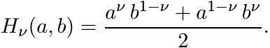 (4.65)
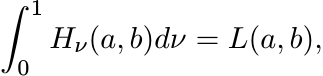
We call these the Heinz means. Notice that Hν = H1−ν, H1/2 is the geometric mean, and H0 = H1 is the arithmetic mean. Thus, the family Hν interpolates between the geometric and the arithmetic mean. Each Hν satisfies conditions (i)–(vi) for means.
4.5.5 Exercise
(i) For fixed positive numbers a and b, Hν(a, b) is a convex function of ν in the interval [0, 1], and attains its minimum at ν = 1/2.
Thus
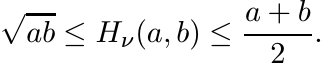 (4.66)
(ii) Show that
 (4.67)
and use this to prove the inequality (4.3).
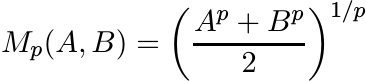
For −∞ ≤ p ≤ ∞ let
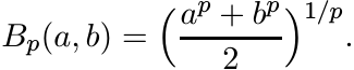 (4.68)
These are called the power means or the binomial means. Here it is understood that
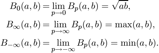
The arithmetic and the harmonic means are included in this family. Properties (i)–(vi) of means may readily be verified for this family.
In Section 4.1 we defined the geometric mean A#B by using the congruence ΓA−1/2 to reduce the pair (A, B) to the commuting pair (I, A−1/2BA−1/2). A similar procedure may be used for the other means. Given a mean M on positive numbers, let
4.5.6 Exercise
From properties (i)–(vi) of M deduce that the function f on ![]() has the following properties:
has the following properties:
(i) f(1) = 1,
(ii) xf(x−1) = f(x),
(iii) f is monotone increasing,
(iv) f is continuous,
(v) f(x) ≤ 1 for 0 < x ≤ 1, and f(x) ≥ 1 for x ≥ 1.
4.5.7 Exercise
Let f be a map of ![]() into itself satisfying the properties (i)–(v) given in Exercise
4.5.6. For positive numbers a and b let
into itself satisfying the properties (i)–(v) given in Exercise
4.5.6. For positive numbers a and b let
Show that M is a mean.
Given a mean M(a, b) on positive numbers let f(x) be the function associated with it by the relation (4.69). For positive matrices A and B let
When ![]() this formula gives the geometric mean A#B defined in (4.10). Does this procedure
always lead to an operator mean satisfying conditions (i)–(vi)? For the geometric
mean we verified its symmetry by an indirect argument. The next proposition says
that such symmetry is a general fact.
this formula gives the geometric mean A#B defined in (4.10). Does this procedure
always lead to an operator mean satisfying conditions (i)–(vi)? For the geometric
mean we verified its symmetry by an indirect argument. The next proposition says
that such symmetry is a general fact.
4.5.8 Proposition
Let M(A, B) be defined by (4.71). Then for all A and B
Proof. We have to show that
If A−1/2B1/2 = UP is the polar decomposition, then B1/2A−1/2 = PU∗ and B−1/2A1/2 = P−1U∗. The left-hand side of (4.73) is, therefore, equal to
The right-hand side of (4.73) is equal to
So, (4.73) will be proved if we show that f(P2) = Pf(P−2)P. This follows from the fact that for every x we have f(x2) = x2f(x−2) as shown in Exercise 4.5.6. ■
4.5.9 Exercise
Show that M(A, B) defined by (4.71) is invariant under congruence; i.e.,
for every invertible matrix X. [Hint: Use the polar decomposition.]
Our next concern is whether M(A, B) defined by (4.71) is monotone in the variables A and B. This is so provided the function f is operator monotone. In this case monotonicity in B is evident from the formula (4.71). By symmetry it is monotone in A as well.
For the means that we have considered in this chapter the function f is given by
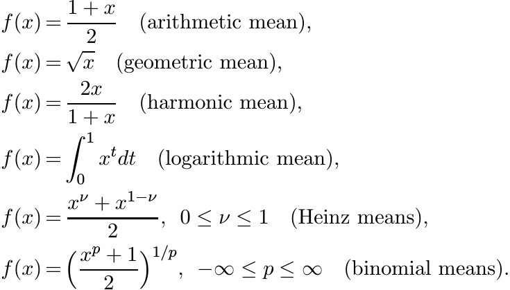
The first five functions in this list are operator monotone. The last enjoys this property only for some values of p.
4.5.10 Exercise
Let f be an operator monotone function on (0, ∞). Then the function g(x) = [f(xp)]1/p is operator monotone for 0 < p ≤ 1. [It may be helpful, in proving this, to use a theorem of Loewner that says f is operator monotone if and only if it has an analytic continuation mapping the upper half-plane into itself. See MA Chapter V.]
4.5.11 Exercise
Show that the function
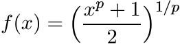
is operator monotone if and only if −1 ≤ p ≤ 1.
Thus the binomial means Bp(a, b) defined by (4.68) lead to matrix means satisfying all our requirements if and only if −1 ≤ p ≤ 1. The mean B0(a, b) leads to the geometric mean A#B.
The logarithmic mean is important in different contexts, one of them being heat flow. We explain this briefly. Heat transfer by steady unidirectional conduction is governed by Fourier’s law. If the direction of heat flow is along the x-axis, this law says
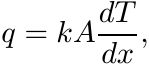 (4.74)
where q is the rate of heat flow along the x-axis across an area A normal to the x-axis, dT/dx is the temperature gradient along the x direction, and k is a constant called thermal conductivity of the material through which the heat is flowing.
The cross-sectional area A may be constant, as for example in a cube. More often, as in the case of a fluid traveling in a pipe, it is a variable. In such cases it is convenient for engineering calculations to write (4.74) as
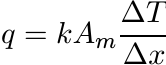 (4.75)
where Am is the mean cross section of the body between two points at distance ∆x along the x-axis and ∆T is the difference of temperatures at these two points. For example, in the case of a body with uniformly tapering rectangular cross section, Am is the arithmetic mean of the two boundary areas A1 and A2.
A very common situation is that of a liquid flowing through a long hollow cylinder (like a pipe). Here heat flows through the sides of the cylinder in a radial direction perpendicular to the axis of the cylinder. The cross sectional area in this case is proportional to the distance from the centre.
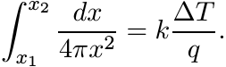
Consider the section of the cylinder bounded by two concentric cylinders at distances x1 and x2 from the centre. Total heat flow across this section given by (4.74) is
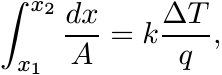 (4.76)
where A = 2πxL, L being the length of the cylinder. This shows that
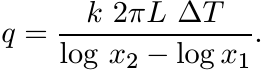
If we wish to write it in the form (4.75) with ∆x = x2 − x1, then we must have
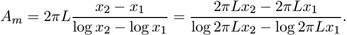
In other words,
the logarithmic mean of the two areas bounding the section under consideration. In the chemical engineering literature this is called the logarithmic mean area.
If instead of a hollow cylinder we consider a hollow sphere, then the cross-sectional area is proportional to the square of the distance from the center. In this case we get from (4.76)
The reader can check that in this case
the geometric mean of the two areas bounding the annular section under consideration.
In Chapter 6 we will see that the inequality between the geometric and the logarithmic mean plays a fundamental role in differential geometry.
4.6 NOTES AND REFERENCES
The parallel sum (4.4) was introduced by W. N. Anderson and R. J. Duffin, Series and parallel addition of matrices, J. Math. Anal. Appl., 26 (1969) 576–594. They also proved some of the basic properties of this object like monotonicity and concavity, and the arithmetic-harmonic mean inequality. Several other operations corresponding to different kinds of electrical networks were defined following the parallel sum. See W. N. Anderson and G. E. Trapp, Matrix operations induced by electrical network connections—a survey, in Constructive Approaches to Mathematical Models, Academic Press, 1979, pp. 53–73.
The geometric mean formula (4.10) and some of its properties like (4.13) are given in W. Pusz and S. L. Woronowicz, Functional calculus for sesquilinear forms and the purification map, Rep. Math. Phys., 8 (1975) 159–170. The notations and the language of this paper are different from ours. It was in the beautiful paper T. Ando, Concavity of certain maps on positive definite matrices and applications to Hadamard products, Linear Algebra Appl., 26 (1979) 203–241, that several concepts were clearly stated, many basic properties demonstrated, and the power of the idea illustrated through several applications. The interplay between means and positive linear maps clearly comes out in this paper, concavity and convexity of various maps are studied, a new proof of Lieb’s theorem 4.27 is given and many new kinds of inequalities for the Schur product are obtained. This paper gave a lot of impetus to the study of matrix means, and of matrix inequalities in general.
W. N. Anderson and G. E. Trapp, Operator means and electrical networks, in Proc. 1980 IEEE International Symposium on Circuits and Systems, pointed out that A#B is the positive solution of the Riccati equation (4.11). They also drew attention to the matrix in Proposition 4.1.9. This had been studied in H. J. Carlin and G. A. Noble, Circuit properties of coupled dispersive lines with applications to wave guide modelling, in Proc. Network and Signal Theory, J. K. Skwirzynski and J. O. Scanlan, eds., Peter Pergrinus, 1973, pp. 258–269. Note that this paper predates the one by Pusz and Woronowicz.
An axiomatic theory of matrix means was developed in F. Kubo and T. Ando, Means of positive linear operators, Math. Ann., 246 (1980) 205–224. Here it is shown that there is a one-to-one correspondence between matrix monotone functions and matrix means. This is implicit in some of our discussion in Section 4.5.
A notion of geometric mean different from ours is introduced and studied by M. Fiedler and V. Pták, A new positive definite geometric mean of two positive definite matrices, Linear Algebra Appl., 251 (1997) 1–20. This paper contains a discussion of the mean A#B as well.
Entropy is an important notion in statistical mechanics and in information theory. Both of these subjects have their classical and quantum versions. Eminently readable introductions are given by E. H. Lieb and J. Yngvason, A guide to entropy and the second law of thermodynamics, Notices Am. Math. Soc., 45 (1998) 571–581, and in other articles by these two authors such as The mathematical structure of the second law of thermodynamics, in Current Developments in Mathematics, 2001, International Press, 2002. The two articles by A. Wehrl, General properties of entropy, Rev. Mod. Phys., 50 (1978) 221–260, and The many facets of entropy, Rep. Math. Phys., 30 (1991) 119–129, are comprehensive surveys of various aspects of the subject. The text by M. Ohya and D. Petz, Quantum Entropy and Its Use, Springer, 1993, is another resource. The book by M. A. Nielsen and I. L. Chuang, Quantum Computation and Quantum Information, Cambridge University Press, 2000, reflects the renewed vigorous interest in this topic because of the possibility of new significant applications to information technology.
Let (p1, . . . , pn) be a probability vector; i.e., pi ≥ 0 and ![]() = 1. C. Shannon,
Mathematical theory of communication, Bell Syst. Tech. J., 27 (1948) 379–423, introduced
the function S(p1, . . . , pn) =
= 1. C. Shannon,
Mathematical theory of communication, Bell Syst. Tech. J., 27 (1948) 379–423, introduced
the function S(p1, . . . , pn) = ![]() as a measure of “average lack of information” in
a statistical experiment with n possible outcomes occurring with probabilities p1,
. . . , pn. The quantum analogue of a probability vector is a density matrix A; i.e.,
A ≥ O and tr A = 1. The quantum entropy function S(A) = −tr A log A was defined
by J. von Neumann, Thermodynamik quantenmechanischer Gesamtheiten, Göttingen Nachr.,
1927, pp. 273–291; see also Chapter 5 of his book Mathematical Foundations of Quantum
Mechanics, Princeton University Press, 1955. Thus von Neumann’s definition preceded
Shannon’s. There were strong motivations for the former because of the work of nineteenth-century
physicists, especially L. Boltzmann.
as a measure of “average lack of information” in
a statistical experiment with n possible outcomes occurring with probabilities p1,
. . . , pn. The quantum analogue of a probability vector is a density matrix A; i.e.,
A ≥ O and tr A = 1. The quantum entropy function S(A) = −tr A log A was defined
by J. von Neumann, Thermodynamik quantenmechanischer Gesamtheiten, Göttingen Nachr.,
1927, pp. 273–291; see also Chapter 5 of his book Mathematical Foundations of Quantum
Mechanics, Princeton University Press, 1955. Thus von Neumann’s definition preceded
Shannon’s. There were strong motivations for the former because of the work of nineteenth-century
physicists, especially L. Boltzmann.
Theorem 4.3.3 was proved in E. H. Lieb, Convex trace functions and the Wigner-Yanase-Dyson conjecture, Adv. Math., 11 (1973) 267–288. Because of its fundamental interest and importance, several different proofs appeared soon after Lieb’s paper. One immediate major application of this theorem was made in the proof of Theorem 4.3.14 by E. H. Lieb and M. B. Ruskai, A fundamental property of quantum-mechanical entropy, Phys. Rev. Lett., 30 (1973) 434–436, and Proof of the strong subadditivity of quantum-mechanical entropy, J. Math. Phys., 14 (1973) 1938–1941. Several papers of Lieb are conveniently collected in Inequalities, Selecta of Elliot H. Lieb, M. Loss and M. B. Ruskai eds., Springer, 2002. The matrix-friendly proof of Theorem 4.3.14 is adopted from R. Bhatia, Partial traces and entropy inequalities, Linear Algebra Appl., 375 (2003) 211–220.
Three papers of G. Lindblad, Entropy, information and quantum measurements, Commun. Math. Phys., 33 (1973) 305–322, Expectations and entropy inequalities for finite quantum systems, ibid. 39 (1974) 111–119, and Completely positive maps and entropy inequalities, ibid. 40 (1975) 147–151, explore various convexity properties of entropy and their interrelations. For example, the equivalence of Theorems 4.3.5 and 4.3.14 is noted in the second paper and the inequality (4.48) is proved in the third.
In the context of quantum statistical mechanics the tensor product operation represents the physical notion of putting a system in a larger system. In quantum information theory it is used to represent the notion of entanglement of states. These considerations have led to several problems very similar to the ones discussed in Section 4.3. We mention one of these as an illustrative example. Let Φ be a completely positive trace-preserving (CPTP) map on Mn. The minimal entropy of the “quantum channel” Φ is defined as
It is conjectured that
for any two CPTP maps Φ1 and Φ2. See P. W. Shor, Equivalence of additivity questions in quantum information theory, Commun. Math. Phys., 246 (2004) 453–472 for a statement of several problems of this type and their importance.
Furuta’s inequality was proved by T. Furuta, A ≥ B ≥ O assures (BrApBr)1/q ≥ B(p+2r)/q for r ≥ 0, p ≥ 0, q ≥ 1 with (1 + 2r)q ≥ p + 2r, Proc. Am. Math. Soc. 101 (1987) 85–88. This paper sparked off several others giving different proofs, extensions, and applications. For example, T. Ando, On some operator inequalities, Math. Ann., 279 (1987) 157–159, showed that if A ≥ B, then e−tA#etB ≤ I for all t ≥ 0. It was pointed out at the beginning of Section 4.4 that A ≥ B ≥ O does not imply A2 ≥ B2 but it does imply the weaker inequality (BA2B)1/2 ≥ B2. This can be restated as A−2#B2 ≤ I. In a similar vein, A ≥ B does not imply eA ≥ eB but it does imply e−A#eB ≤ I. It is not surprising that Furuta’s inequality is related to the theory of means and to properties of matrix exponential and logarithm functions.
The name “Heinz means” for (4.65) is not standard usage. We have called them so because of the famous inequalities of E. Heinz (proved in Chapter 5). The means (4.68) have been studied extensively. See for example, G. H. Hardy, J. E. Littlewood, and G. Polya, Inequalities, Second Edition, Cambridge University Press, 1952. The matrix analogues
are analysed in K. V. Bhagwat and R. Subramanian, Inequalities between means of
positive operators, Math. Proc. Cambridge Philos. Soc., 83 (1978) 393–401. It is
noted there that the limiting value ![]() . We have seen that this is not a suitable definition
of the geometric mean of A and B.
. We have seen that this is not a suitable definition
of the geometric mean of A and B.
A very interesting article on the matrix geometric mean is J. D. Lawson and Y. Lim, The geometric mean, matrices, metrics, and more, Am. Math. Monthly 108 (2001) 797–812. The importance of the logarithmic mean in engineering problems is discussed, for example, in W. H. McAdams, Heat Transmission, Third Edition, McGraw Hill, 1954.