
Our customer for this chapter is a mid-size company that manufactures sporting goods and related accessories and, more recently, sports-related clothing. Their customers are large retail companies around the world.
The information available is restricted by the current enterprise resource planning (ERP) systems’ functionality, and it is difficult for end users to access operational information. Building new reports to answer business questions is a slow and costly process, and the promise of “end-user reporting” has never been realized because there are multiple systems, and in each system information is spread across multiple tables and requires expert knowledge to answer simple business questions.
This has led to the following issues:
-
The manufacturer is falling behind competitively because business processes cannot keep up with change. Initiatives such as improvements in on-time deliveries and understanding the real impact of complex customer discounting structures are information intensive and are almost impossible to achieve across the business in a timely and cost-effective way.
-
IT is finding it difficult to give people the information that they need to keep up with a changing business environment, and with the complexity of the different ERP systems, it is taking longer to deliver solutions. It is also expensive to answer simple one-off, what-if type questions.
-
Using the ERP systems for reporting is adversely affecting the transaction systems’ performance during peak reporting periods.
We will build a data warehouse that consolidates the data from the ERP systems and other sources to enable new types of analyses and reduce the cost and complexity of delivering information. With our business value-based approach, we will focus on building the necessary functionality to support the highest-priority business objectives while providing a platform for future enhancements.
The high-level requirements to support the key business objectives are as follows:
-
Sales reporting and performance tracking. The business needs timely and flexible access to sales information such as units shipped and revenue, including the ability to understand sales performance by territory, by product, and by customer. Ultimately, the goal is to track the actual sales achieved against the targets for each sales territory.
-
Profitability. A key business driver is that the solution needs to include enough information to enable profitability analysis. This comprises information such as manufacturing and shipping costs and any discounts offered to customers. This will enable the business to understand profitability of product lines as well as types of customers and to optimize the mix of products and customers.
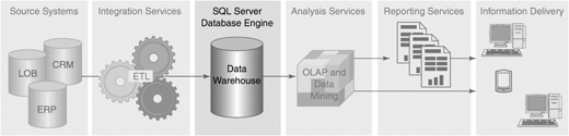
The primary component of our solution is a data warehouse database that receives information from the source systems, as shown in Figure 3-1. We will focus in this phase of the project on building a database to support the requirements, and we will build the data integration process and more complex analytics in the following chapters.
The solution will deliver the following benefits to the client:
The primary goal of dimensional data modeling is to produce a simple, consistent model that is expressed in the users’ own language and will enable them to easily access information. A common challenge when building BI solutions is that there are often so many areas in the business that have interesting information, you really need to resist trying to produce an initial data model that covers everything in the whole business. The key tenet of our approach is that you should carefully define the areas you will be focusing on delivering so that they align with the objectives and can deliver actual business value (something that has been in short supply in many large data warehouse projects).
The business requirements describe our area of focus as sales and profitability reporting. We will deliver the data model to support these requirements, but design the dimensions so that they can become the “one version of the truth” that is eventually used in other areas of the business such as analyzing manufacturing scheduling or loss analysis.
As it turns out, defining the exact business process that we need to model is a bit tricky. To handle sales reporting and profitability, we need to know information from manufacturing (what is the actual cost of the manufactured products), ordering and invoicing (how much did we charge this customer taking into account discounts and other contract terms), and delivery (did the goods arrive on time and in good condition). This data is almost certainly stored in different tables in the transaction systems, and in fact may be in separate systems altogether.
TIP:
Do Not Constrain the DW Design by the OLTP Design
Designing data warehouse fact tables that do not necessarily map to a single transaction table (such as InvoiceLineItem) is a common feature of data warehouses and shouldn’t worry you. The trap to avoid is designing your data warehouse schema by looking at the transaction systems. You should first focus on the end users and how they understand the information.
The business process that spans all these areas is often known as “shipments,” and it includes so much useful information that having shipments data in the data warehouse is one of the most important and powerful capabilities for manufacturing.
Now that we have identified the shipments business process, the next question that we are faced with is the grain of information required. Do we need daily totals of all shipments for the day, or would monthly balances suffice? Do we need to know which individual products were involved, or can we summarize the information by category?
In some ways, this data modeling question of granularity is the easiest to resolve because the answer is always the same: You should strive to always use the most detailed level of information that is available. In the shipments example, we need to store a record for each individual line item shipped, including the customer that it was shipped to, the product UPC, the quantity shipped, and all the other information we can find in this area.
In the bad old days before technology caught up with our BI ambitions, a lot of compromises needed to be made to avoid large data volumes, which usually involved summarizing the data. A lack of detailed information leads to all kinds of problems in data warehouses—for example, if we store the shipments summarized by product group, how do I find out whether yellow products are more popular than green ones? We need the product detail-level information to figure that out. Today, modern hardware and SQL Server 2005 easily support detail-level information without special handling in all but the most demanding of applications. (See Chapter 11, “Very Large Data Warehouses,” for more information on dealing with very large data warehouses.)
This is probably the most important dimensional modeling lesson that we can share: A single fact table must never contain measures at different levels of granularity. This sounds like it should be easy to achieve, but some common pitfalls can trip you up, usually related to budget or forecast information. For example, business users often want to compare the actual measure (such as actual quantity shipped) with a forecast or budget measure (such as budget quantity). Budgets are usually produced at a higher level of granularity (for example, planned monthly sales per product group), and therefore should never be put into the same fact table that stores the detail-level transactions. If you find measures at different levels of granularity, you must create a separate fact table at the right level.
As discussed in Chapter 1, “Introduction to Business Intelligence,” the heart of the dimensional approach is to provide information to users in the ways they would like to look at it. One of the best ways to start identifying dimensions is to take note every time anyone says the word by. For example, we need to see sales by manufacturing plant, and we need to look at deliveries by the method they were shipped to see which method is more cost-effective. Each of these “bys” is a candidate for a dimension.
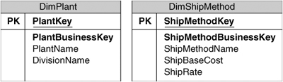
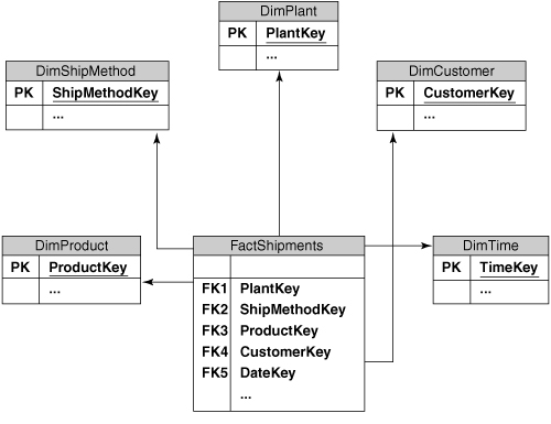
Out of the interviews with the business users, we can so far add two dimensions to our data model, as shown in Figure 3-2: Plant, which identifies where the product in a shipment was manufactured and shipped from; and Ship Method, which indicates the method used to ship the product.
One of the main dimensions in this data warehouse contains the Product information. Products can be grouped into subcategories and categories, and each Product record can contain many descriptive attributes that are useful for understanding sales and profitability, such as Color or Size. To make it easy to load the Product information and to improve the efficiency of the queries used to load the cube, we will “snowflake” the dimension and create three separate tables, as shown in Figure 3-3. This is the first example of the design decision-making process that we outlined in Chapter 1; that is, when we have a dimension table with an obvious hierarchy, we can renormalize or snowflake the dimension into a separate table for each level in the hierarchy.
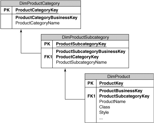
Note that every snowflake dimension table still follows the rule for surrogate keys, which is that all primary keys used in a data warehouse are surrogate keys and these are the only keys used to describe relationships between data warehouse tables. In the case of the Product Subcategory table, you can see that we have used the ProductCategoryKey for the relationship with the Product Category table.
The manufacturer in our example has an interesting issue with Products—their original business was the manufacture of sporting goods and related equipment, but several years ago they acquired another company with several plants that manufacture sports-related clothing. The two divisions in the company have separate ERP systems and totally separate product lines. In a data warehouse, we want a single Product dimension that is the only version of the truth.
Even though the two ERP systems might have different ways of storing the product information and we will have to perform some calisthenics in the extraction, transformation, and loading (ETL) process, we must reconcile these differences to create a single Product dimension. The design that we must avoid is having two separate product dimensions that map back to the source systems; otherwise, it will be difficult for users to include all the available information in their analysis.
The next interesting area in our data model is Customers. The manufacturer does not sell direct to consumers but only to retailers, so each customer record contains information about a company that does business with the manufacturer. In addition to attributes such as customer type (such as Retailer or Distributor), one of the most important sources of customer attributes is geographical information.
Each customer is physically located at an address, and you can see how users would find it useful to be able to group data by the customer’s state or province, or even drill down to the city level. In addition to this natural “geographical” hierarchy, most companies also divide up geographical areas into “sales territories.” These sales territories might not translate perfectly to the natural geographical structures such as state or province, because a company’s rules governing which cities or customers fall into which sales territories may be complex or arbitrary. So, sometimes end users will want to see information grouped by physical geography and sometimes grouped by sales territories.
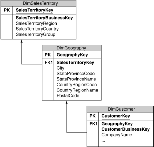
In our data model, we will extract the physical geographical information from the customer record and move it a Geography dimension, which will have one record for each Zip/Postal Code. This dimension record will contain all the natural geographical information such as state or province name, and each Customer record will have a GeographyKey column that contains the surrogate key of the appropriate Geography record. We will also create a separate Sales Territory dimension, and extend the Geography dimension so that every record relates to a particular sales territory, as shown in Figure 3-4.
By far the most common way of looking at information in data warehouses is analyzing information in different time periods. Users might want to see shipments for the current month, or year-to-date shipments, or compare the current period with the same period last year. Every shipment transaction has one or more dates associated with it (such as date ordered and date shipped), and we need to allow these dates to be used to group the shipments together.
The first thing that we need to determine is the level of detail required for our fact table. The shipments fact includes the actual date of the transaction, so we need day-level information rather than just weekly or monthly summaries.
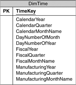
Because most modern applications include extensive functions for interpreting date fields, it might seem that we don’t need to create an actual dimension table for Time. As it turns out, a physical table that contains a record for each day, as shown in Figure 3-5, is very useful. Not only can we include the obvious attributes on every day such as the name of the day or the year; we can also get creative about providing analytical columns. For example, we could include a flag that shows which days are holidays so that users can select those days for special analysis. When we have lots of descriptive attributes in the table, we can use the analytical capabilities of Analysis Services to provide the capability of selecting complicated ranges such as year-to-date.
TIP:
Do Not Include Hourly or Minute-Level Records
If it turned out to be useful to know the actual time that a transaction occurred rather than just the day, you might think that we should just add more detailed information to the Time dimension table. This entails a number of problems; not only will this increase the size of the dimension (storing records at the minute level would mean 1,440 records per day!), but from an analytical point of view, it is not very useful.
Users most likely would want to select a date range and then see how transactions varied at different times of the day. The best way to support this is to leave the Time dimension at the day level (probably renamed Date for clarity) and create a separate dimension for Time Of Day. This would contain only one record for each time period, such as a total of 1,440 records for a minute-level Time Of Day dimension.
The other useful feature that you can provide in a Time dimension is support for multiple ways of grouping dates. In addition to looking at a natural calendar hierarchy such as year or month, most businesses want the ability to see fiscal periods. We can accommodate this by including the fiscal year (which usually starts on a different day to the natural calendar) and fiscal month on every daily record in addition to the standard calendar year and month. This could also be extended to support manufacturing calendars, which consist of 13 periods of exactly the same size made up of four weeks each.
Now that we have identified the different ways that users will want to see the information, we can move on to our next modeling question: What numbers will the user want to analyze?
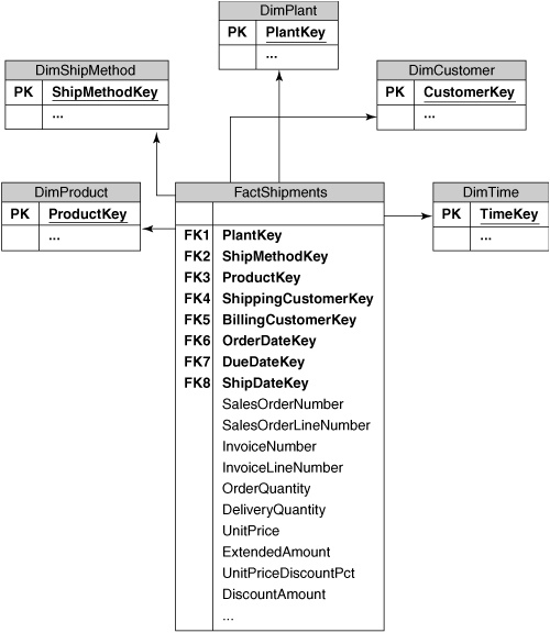
All the information that we want to analyze, such as sales amounts, costs, or discounts, will end up on our fact table. Now that we have identified the grain of this fact table and designed the dimensions that we will be using, we can move on to building a list of numeric measures for the table. At this point in the design process, the fact table looks like Figure 3-6.
TIP:
The Importance of Clarifying Terms
Most data modelers find out early on that trying to do data modeling without a good understanding of the underlying business is a risky undertaking. People often tend to use different terms for the same concept depending on their specific area of the business, or use the same terms for very different concepts in different business areas. It is important to recognize this and take extra care to clarify terms even if they sound like commonsense concepts.
Ultimately, the source for all the measures in a fact table will be a transaction table in the ERP systems, but it would be a mistake to start from the ERP schema to identify measures. As previously described, on-line transaction processing (OLTP) systems have normalization as a primary driver of their designs, whereas much of the information in data warehouses is derived. A better approach is to start from the business questions that the users need to answer and then attempt to build a list of measures that will be required to provide the answers. Some of this information might turn out to not be available in the ERP systems, but at least these issues can then be identified to the ERP team.
For example, an obvious candidate measure is the quantity of the product item that the customer ordered, but equally important for analysis is a measure that describes the actual quantity that was delivered, taking into account any breakages or errors in the shipping process. We can add both Quantity Ordered as well as Quantity Delivered measures to the fact table. The business requirements also lead us to add other numeric columns to support profitability analysis, such as discounts and manufacturing costs.
All the measures that we have looked at so far are fully additive—that is, whether we are looking at a product group total for the last year or a single customer’s transactions in a week, all we have to do is sum up the numbers on the fact table to arrive at the correct answer. Not all numbers are quite so obliging, however; for example, whereas the quantity of product sold in a shipment record is additive, the unit price is not. If you imagine what would happen if we looked at a year’s total of all the unit prices in the Shipments table, you can see that this would not produce a sensible measure. In the case of unit prices that might increase or decrease over time, and other “rate” types of measures, the usual way of looking at the information is by taking an average over the time period we are querying.
The same logic usually applies to “balance” types of measures such as inventory balances, where either the average balance or the latest balance in the selected time period is much more meaningful than a total. These measures are known as partially additive or semi-additive, because we can sum them up along dimensions such as Customer or Product, but not across other dimensions such as the Time dimension.
It is often possible to transform “rate” measures into fully additive measures just by multiplying by the corresponding measure such as quantity. This will produce a fully additive measure such as Revenue rather than a semi-additive measure such as Unit Price. If you want to actually include a semi-additive measure, you can simply add the numeric column to the fact table—Analysis Services cubes can be set up so that the appropriate summary calculation is performed for semi-additive measures.
Most of the relationships between dimension tables and the fact table are simple and easy to model. For example, every shipment has a method of shipping, so we can just add the ShipMethodKey to the fact table. Not all dimensions are quite so easy to handle, however; the Customer and Time dimensions in the manufacturing solution have more complex relationships with the fact table.
Every shipment that we make is sent to a specific customer, so we could just add a CustomerKey column to the fact table. However, because of the intricate corporate hierarchies that the manufacturer needs to deal with, the bill for the shipment might be sent to a different corporate entity (such as a parent company) than the customer that received the shipment. It is easy to find business requirements that would require both of these concepts, such as a financial analysis by the billing customer and a logistics or shipping analysis by the shipping customer. To accommodate this, we can simply add both ShippingCustomerKey and BillingCustomerKey columns to the fact table and populate them accordingly.
The Time dimension has a similar requirement. Depending on the analysis, users might want to see the shipments by the date that the order was placed, or the date that it was shipped, or even to compare the date actually shipped with the date that the shipment was due to take place. Each of these requires a new dimension key column on the fact table, as shown in Figure 3-7.
The columns that we have added to the fact table so far are either dimension keys or numeric measures. Often, you must include some columns in an analysis that do not fall into either of these neat categories. A common example of this is Invoice Number. It would make no sense to consider this a numeric measure because we cannot sum or average it; and because there are probably many thousands of invoices and no real descriptive attributes to group them by, it is not really a dimension either. All the interesting information on an invoice has already been added to the fact table in the form of dimensions such as Customer and Product.
The Invoice Number would still be useful in many analyses, however, especially when a user has drilled down to a level of detail that includes only a few invoices and wants to see the full details of each. Adding this kind of column to a fact table is usually known as a degenerate dimension, because it is basically a dimension with only one column, which is the business key.
In this section, we focus on building the relational tables to support the dimensional model that we have designed in the previous section and discuss some of the common design decisions you need to make when building data warehouse tables. The following chapters cover the details of loading the data from the source systems and building Analysis Services cubes to present the information to end users.
Although some minor differences exist in the table designs for different business solutions, most dimension and fact table structures usually follow a strikingly similar pattern. Some standard ways of approaching the requirements for a well-performing data warehouse are common across most modern databases, including SQL Server 2005. We can start by building the Ship Method dimension table to demonstrate the approach.
As described in Chapter 1, every dimension table has a surrogate key column that is generated within the data warehouse and uniquely identifies the dimension record. In SQL Server databases, we can implement surrogate keys using a concept called identity columns.
The first column that we will add to the dimension table is called ShipMethodKey (see the sidebar “Using Naming Standards”), which is the surrogate key for the table. All surrogate keys in our databases are declared as integer fields with the IDENTITY property turned on. This means that there is no need to specify a value for this column. The database will generate a unique incremental value every time a new row is added to the table.
The manufacturer has assigned a code for every method of shipping products to their customers, such as OSD for Overseas Deluxe shipping. Although we are internally using the surrogate key as the only identifier for shipping methods, we still need to store the original shipping code along with every record. This code will be used to translate the shipping codes in information received from source systems and is known as the business key.
Unlike surrogate keys, every business key in the data warehouse may have a different data type, so we must make a decision for each dimension table. The shipping method codes are currently three-character identifiers in the source systems, so char(3) would probably be a good candidate here. Some data warehouse designers like to add some additional space into codes to cater for any future systems that might need to be integrated that use longer codes; but because it is generally a trivial exercise to change this size if it becomes necessary (especially in dimension tables, which are usually much smaller than fact tables), this is certainly optional.
Business keys tend to have a wide range of names in source systems (such as CustomerNumber, ShippingMethodCode, or ProductID), so we will pick the nice consistent naming convention of using ShipMethodBusinessKey and follow this for all our business keys. When creating the column, remember that business keys should generally not allow nulls.
We will also add a unique key constraint for the ShipMethodBusinessKey column and for all the business key columns in our other dimension tables. Because we will be using the business key to look up records from the source system, the unique key constraint will ensure that we don’t have any duplicates that would make this process fail. (See Chapter 8, “Managing Changing Data,” for a common exception to the rule for unique business keys.)
The unique key constraint that we added to the business key will also provide an index on the column, and we will pick this index as the clustered index for the dimension table. This means that the data in the table will be physically arranged in order of the business key, which will improve performance when we need to fetch the dimension record based on the business key. For example, when a dimension record is received from the source systems, the ETL process will need to do a lookup using the business key to determine whether the record is new or is an existing record that has been changed.
Data warehouses that are used primarily as a consistent store to load Analysis Services cubes actually need little indexing because all the end-user querying takes place against the cube, but a careful indexing design that includes the surrogate keys used for relational joins will improve the performance for applications that run queries directly against the data warehouse, such as relational reporting.
All the other columns in our Ship Method dimension table are descriptive attributes that can be used to analyze the information. During the data modeling stage, we will always try to include as many of these attributes as possible to increase the usefulness of our data warehouse. Attributes have different data types depending on the type of information (such as the currency shipping cost and rates on the Ship Method dimension), but many of them contain textual information.
When you are building a new data warehouse, you will often find patterns in the data types you are using for attributes, such as having some columns with a short description of up to 50 characters and other columns with a longer description of 100 characters. A useful technique is to take advantage of SQL Server’s user-defined types feature to create special data types for common categories of columns, such as ShortDesc and LongDesc. This will standardize your approach for creating attributes, and make it easier to change the columns if the approach changes.
As discussed in the Preface, the Quick Start exercises are intended to get you started with using the SQL Server tools to implement the technical solution we are discussing. In this Quick Start, we create a new data warehouse database and add the first dimension table, DimShipMethod.
-
Open the SQL Server Management Studio.
-
If you are prompted to connect to your database server, select your authentication type and click Connect. If this is the first time you are opening the Management Studio, choose Connect Object Explorer from the File menu, choose Database Engine as the server type, and select your database server name.
-
To create a new database, right-click the Databases folder in the Object Explorer and select New Database; then specify a name for your database, such as ManufacturingDW, and click OK to create it.
-
In the Object Explorer pane, expand the Databases folder and find your new database; then expand the database folder to see the object type folders, such as Database Diagrams and Tables.
-
To create the new dimension table, right-click Tables and choose New Table. A new window will open up in Management Studio to allow you to specify the columns and other settings. (You are prompted to name the table only when you save it.)
-
For the first column, specify ShipMethodKey as the name and
intas the data type, and uncheck the Allow Nulls box. In the column properties, open up the Identity Specification section and set the (Is Identity) property to Yes. -
To specify the new column as the primary key, right-click the ShipMethodKey column and choose Set Primary Key.
-
In the next grid row, add the ShipMethodBusinessKey column with a data type of char(3), and uncheck the Allow Nulls box.
-
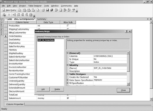
Right-click the table and choose Indexes/Keys. You need to change the Create As Clustered property of the existing primary key to be No, because each table can only have one clustered index, and we will be adding one for the business key instead.
-
To add a unique key constraint for the business key, click the Add button to create a new index. For the Columns property, select ShipMethodBusinessKey, change the Type property to Unique Key, and change the Create As Clustered property to Yes. Click the Close button to return to the table designer.
-
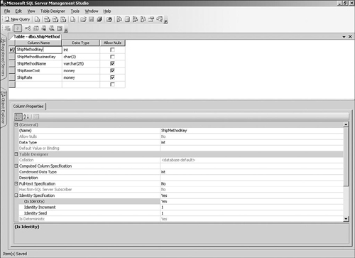
Add the other descriptive attributes columns for the Ship Method dimension (see the data model), using
varchar(25)as the data type for the ship method name andmoneyfor the other columns, as shown in Figure 3-8. -
Click the Save button on the toolbar and specify DimShipMethod as the table name.
As discussed in the “Data Model” section, the Time table has a record for each time period that we are measuring, which is per day for the manufacturing example. The table consists of descriptive attributes to support the various hierarchies such as Calendar and Fiscal, as well as other descriptive attributes such as the day number of the year or whether the day is a public holiday.
Although we could follow the usual convention of using an automatically generated integer surrogate key, it is often convenient for Time dimension tables to use an actual DateTime column as the primary key. Because the actual date is the value that is known to the source systems, this is basically the equivalent of using the business key rather than a generated surrogate. This violates the design guideline of always using a surrogate key, but does make some processes such as loading the fact table easier by avoiding the need to lookup the surrogate key for every date that you encounter.
To support the Analysis Services dimension that we will ultimately build from the Time table, we also need to add an additional unique column for each level in the hierarchies. For example, the Quarter Name attribute contains values such as Quarter 1 and Quarter 2, which are not unique because each year has the same four quarter names. We will add a Quarter key column using the date of the first day in the quarter to provide a unique value for each quarter, such as 01/01/2006, and take the same approach for the other levels such as Year and Month.
After we have finished designing all the dimension tables in the data warehouse, we can move on to the fact tables.
As we have seen in the “Data Model” section, the fact table consists of a column containing the surrogate key for each dimension related to the fact table, as well as columns for the measures that we will be tracking. For the Shipments fact table, we need to add the ProductKey, SalesTerritoryKey, PlantKey, and ShipMethodKey columns. The fact table has two relationships with the Customer dimension, so we need to add separate ShippingCustomerKey and BillingCustomerKey columns to represent this. We also need three date keys (OrderDateKey, DueDateKey, and ShipDateKey) to represent the different dates for each shipment fact.
Most fact tables contain a single record for each distinct combination of the key values, so the logical primary key of the fact table is usually all the dimension keys. However, most information is analyzed with some level of summarization (especially BI solutions using Analysis Services), so it often does not matter whether you have multiple records for the same combination of keys because they will be summed except in some relational reporting scenarios. For this reason, a primary key constraint is usually not added to fact tables, and any potential requirement for avoiding multiple fact records is handled in the data loading (ETL) process.
As described for dimension tables, BI solutions that use Analysis Services cubes to query the information require little indexing in the data warehouse. It is worthwhile, however, to add a clustered index to the fact table, usually on one of the date keys. Because the data will often be queried by a date range, it will be helpful to have the fact data physically arranged in date order. For the Shipments fact table, we will use the earliest date, which is the OrderDateKey, as shown in Figure 3-9. If you are also doing relational reporting from your data warehouse tables, it will probably prove to be beneficial to add indexes for the dimension keys in the fact table because this will speed up joins to the dimension tables.
After the keys, we can add the remaining measure columns using the smallest data type that can contain the measure at the detail level. It is worth being careful with this process because the fact tables are the largest tables in the data warehouse, and properly selected data types can save a lot of space and lead to better performance. The downside of picking a data type that is too small is that at some point, your data loading process will probably fail and need to be restarted after increasing the size of the column.
If we allow client applications such as reporting tools or Analysis Services cubes to directly access the tables in our data warehouse, we run the risk that any future changes that we make might break these applications. Instead, we can create a view for each dimension and fact table in the data warehouse, which makes it easier to change or optimize the underlying database structure without necessarily affecting the client applications that use the database.
You can design views using SQL Server Management Studio, by right-clicking the Views folder under the database and selecting New View. The query designer allows you to add the source tables to the view and select which columns to include, and specify a name when you save the new view.
Referential integrity (RI) is a technique for preserving the relationships between tables and is sometimes used in data warehouse solutions to ensure that every key in the fact table rows has a corresponding dimension row. If your data-loading process tries to add a fact row with a dimension key that does not yet exist, the process will fail because of the RI constraint and ensure that you don’t end up with any mismatched facts.
Good arguments both for and against using referential integrity constraints in the data warehouse exist (and the authors have either used or heard most of them), but we are going to go out on a limb here and state that in a properly architected and managed data warehouse, RI constraints are not required. The primary reason for this is that we always use surrogate keys for dimensions. Because these keys are only known within the data warehouse, a “lookup” step always needs to take place when loading facts to translate business keys into surrogate keys. If this lookup step fails, the new record will either not be added into the fact table or will be added with a special surrogate key that refers to a “Missing” or “Unknown” dimension record.
So, in contrast to OLTP systems where RI is an absolute necessity, a major characteristic of data warehouses that strictly use surrogate keys is that RI is enforced through the data loading process. For this reason, it is not necessary to declare foreign key constraints in the data warehouse. The advantages are that load performance is improved, and the data loading sequence can sometimes be more flexible. The one potential disadvantage is that any errors in your data-loading process are harder to catch until you try to validate the numbers in your data warehouse, so it sometimes proves useful to turn on foreign key constraints during the development process.
It is only when you have exceptions to the rule of always using a surrogate key that you get into trouble, and an especially alert reader might have noticed that we have already broken this rule for one of our tables—the Time dimension. The date keys in our fact table are DateTime columns and do not need to be looked up in the dimension table during load. This means that we will have to add some processing in the data-loading process to check that all the data in the new fact records falls into the date range contained in the Time dimension table, and to trigger a process to have more dates added if not.
If the company you are working with has a database security policy already, you will be able to follow the rules that have been laid out. This section lays out some guidelines for the security decision-making process as it applies to data warehouse databases, but security decisions should always be made with the context of the whole system in mind.
When you connect to a database, SQL Server can either validate your current Windows user account to see whether you have access (which is known as Windows authentication) or prompt you to supply a separate SQL Server login account and password. Windows authentication is usually recommended because it has increased security and it does not require maintaining a separate set of accounts.
We have managed to create a database, add some tables, and specify columns for them, all without worrying about security. How did we manage to have permission to do all of that? If you have installed SQL Server 2005 onto a new server, the reason is probably that you are signed on to the database server as a member of the Administrators group on that machine. When SQL Server is installed, all local Administrators are granted a special right to administer the SQL Server instance, called sysadmin.
Because companies usually don’t want every administrator to have complete control of all the databases on that server, a common approach is to create a new Windows group for database administrators only. SQL Server Management Studio can then be used to add the new database administrators group (under the Security, Logins folder) with the sysadmin role turned on, and then to remove the Administrators group.
TIP:
Log Off After Adding Yourself to a Group
A common mistake that can lead to a moment of panic after making the preceding change is when you have added your own user account to the database administrators group that you created. Just after you remove the Administrators group, you could suddenly be unable to access your databases.
The reason for this is that your Windows group membership only gets refreshed when you log on. To be able to access the database server after you have added yourself to the new database administrators Windows group, you need to log off and back on again so that your credentials are picked up.
The SQL Server security model is flexible and provides extremely granular control over the permissions that users have. You can control which users or groups can view information in a table, whether they can update the information, and other rights such as the ability to execute stored procedures. In all scenarios, we follow the principle of “least privilege,” meaning that we will make sure that users only have the minimum level of permissions that they need to accomplish their tasks.
In the manufacturing data warehouse, we have created views for every dimension and fact table, and most of the data warehouse users will only need to have access to read the information in these views. Because we are using Windows authentication, we can create a Windows group for all users who need read access to the data warehouse’s views. Using groups is much more flexible and easier to maintain than setting up permissions for individual user accounts.
After you have created a Windows group, such as Manufacturing DW Users, you will need to use SQL Server Management Studio to set up the group’s permissions:
-
Open SQL Server Management Studio and connect to the database server.
-
In the Object Explorer pane, find the Security folder and right-click it. Select New Login.
-
Type the name of your group in the Login Name box, or use the Search button to locate the group (for searching, click the Object Types button and include Groups to make sure your group shows up). Select the data warehouse database as the default database.
-
Click the User Mapping page on the left side of the dialog. Check the Map box next to the data warehouse database and click OK.
-
Now that we have created the login, we need to assign the permissions to enable the members of the group to access the views. In the Object Explorer pane, find your database under the Databases folder and open up the Security, Users subfolders.
-
Right-click the name of your group and select Properties. Select the Securables section on the left side of the dialog.
-
Click the Add button and then select Specific objects and click OK. In the Select Objects dialog, click the Object Types button, select Views, and click OK.
-
Click the Browse button to display a list of all the views in your database. Check all the dimension and fact views, and then click OK to close the Browse dialog. Click OK again to close the Select Objects dialog.
-
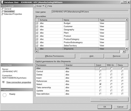
Now that we have added all the views to the list of objects in the Securables section, we need to assign the permissions. Highlight each of the views in turn and check the Grant box for the Select permission (see Figure 3-10). Click OK to close the dialog.
In many BI solutions, users do not access the data warehouse database directly but through an analytical engine such as Analysis Services. In that case, the user account used to connect to the database for the purpose of loading data is often the service account that Analysis Services is using. You can cater for this by adding this service account to the data warehouse users group that you created previously.
Another application that needs access to the database is Integration Services. You can use some flexible options to select which user account is actually used when an Integration Services package is executed to load data, but whatever account is used will need more than just read access to the views. You could use a similar approach to the Quick Start to create a Windows group for data warehouse data loaders, and then instead of granting SELECT permission on individual views, you could add the login to two special database roles: db_datareader and db_datawriter. These roles will allow the data-loading process to read and write data.
No matter how well designed your data warehouse structure is, the success of the data warehouse as a business solution mostly depends on the management process that supports it. Users will only start to integrate the data warehouse into their work when they can rely on a consistently valid source of information that is available whenever they need it.
By the time users get access to the data warehouse, all the information that it contains must have been completely validated. You usually only get one chance to get this right, because deploying a data warehouse that contains incorrect data will inevitably lead the users to question the reliability of the information long after any initial problems have been corrected.
Your development and deployment plan must include testing and an extensive audit of both the numbers and dimension structures. Dimension hierarchies are just as important to validate as numeric measures because incorrect structures will lead to invalid subtotals, which are as damaging as missing or incorrect source data.
If you cannot verify and correct the integrity of some of the data, often the best solution is to leave it out of the data warehouse completely for this release and continue to develop a “phase 2” that contains the additional information. The closer you are to launch, the more politically tricky cutting features in this way becomes, so you should start the auditing process early in the project to identify any potential problems as soon as possible.
In general, SQL Server’s default settings work well for data warehouse databases and don’t require many changes. However, a few areas benefit from adjustment.
Each database has a “Recovery Model” option that you can use to configure how transactions are logged, which can have a major impact on performance. Because most databases are used for capturing transactions, SQL Server defaults to the Full recovery model, which ensures that all transactions are kept in the log, allowing administrators to restore a failed database to any point in time.
For data warehouses, there is often only one large periodic update happening, and the database administrators are in control of when it occurs. For this reason, it is often possible to use the best performing Simple recovery model for data warehouses. In the Simple recovery model, only the data files need to be backed up and not the transaction logs, and log space is automatically reclaimed so space requirements may be reduced. However, databases can only be recovered to the end of the latest backup, so you need to synchronize your backup strategy with your data loads, as described in the “Operations” section.
The issue of where to put the database files can get complicated, especially now with the wide availability of SAN (storage area network) technology. In general, however, a good strategy is to store the data files and log files on physically separate disk drives. For data warehouses, this will improve the performance of your data-load process. It is easier to set the locations of files in the dialog when you first create the database because moving them afterward will require some knowledge of the ALTER DATABASE command.
SQL Server 2005 is generally self-tuning and performs many maintenance tasks automatically. However, you will need to schedule some maintenance tasks yourself, such as backups, checking database integrity and index maintenance tasks such as rebuilds. You can include these tasks in a maintenance plan, which can be scheduled to run automatically.
Maintenance plans in SQL Server 2005 are built on top of Integration Services, which means you have a lot of flexibility when it comes to designing the flow of events. You can also use maintenance plan tasks in regular Integration Services packages, so you could include them as part of your daily or weekly build processes.
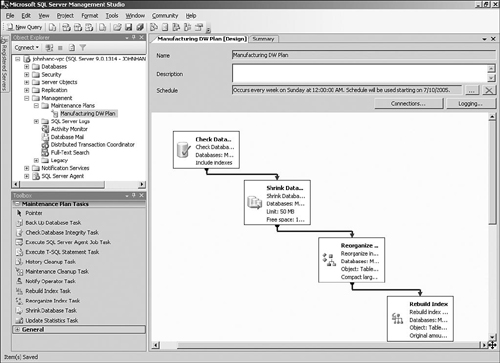
You can design a maintenance plan from scratch, but SQL Server 2005 includes a Maintenance Plan Wizard (see Figure 3-11) that walks you through most of the options to create a fully functional plan. You can access the wizard in the Management Studio’s Object Explorer by right-clicking Maintenance Plans under the Management folder. Before you run the Maintenance Plan Wizard, the SQL Server Agent service must be running, so you might need to run the Surface Area Configuration tool to enable and start this service; by default, it is not enabled.
Because a data warehouse consists of just a database and a set of processes to load the data, it is tempting to ignore all the versioning headaches that application developers have to suffer and just make any required changes directly to the production system. These changes could take the form of adding new columns, modifying the data load procedures, or even adding brand-new business processes.
The problem with that approach is that unless you stick to a clearly defined cycle of develop, test, and release, your data warehouse quality will inevitably suffer. Even when you need to perform the occasional high-priority fix to data loading routines when a bug is identified, this should still be tested in a development environment before deployment.
The so-called backroom activities of loading data, monitoring the database, and performing backups are the key activities required to keep the data warehouse operational. Chapter 4, “Building a Data Integration Process,” covers the load process in detail.
Using the Simple recovery model for our databases means that the transaction logs only contain currently executing transactions, so we only have to concern ourselves with backing up the data files. Because in a data warehouse we are usually in complete control of when data is changed, we can arrange the backups as part of the load process.
Backing up all the data in a database is known as a full backup, and scheduling a full backup on a periodic basis (such as once a week) is a good idea. You should, of course, follow the commonsense rules of handling computer backups, such as making sure they are stored in a separate location from the database to protect against drive failure.
If we are loading data on a daily basis and only performing a full backup once a week, we risk running into trouble if a failure occurs in the middle of the week. One way to solve this is to perform a full backup after every data load, but the issue is that taking a full backup can be a time-consuming exercise and creates large backup files. SQL Server provides a useful feature to handle this that is called differential backups (see Figure 3-12).
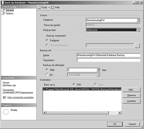
A differential backup only backs up data that has changed since the most recent full backup. (Actually, it backs up slightly more than that because all extents that contain changed pages are backed up, but this is just a technicality.) This leads to smaller backups and faster processing, so a standard approach would be to perform a full backup once a week and differential backups after every data load.
An up-to-date database backup is a valuable tool in case of system failure but also when an issue with the load process occurs. Many data load processes do not operate in a single transaction, so any problems with the load could leave your database in an inconsistent state. To recover the data, you will need a full backup as well as a differential backup that brings the database back to the point just after the most recent successful load.
Database operations staff should also periodically practice restoring the database as a test of the backup procedures, because you don’t want to find out that there is a problem with the procedures when you are facing real data loss.???
Now that we have created a well-structured data warehouse database, we need to look at techniques for loading data from the source systems (covered in Chapter 4) and providing the information to users in a meaningful way (Chapter 5, “Building an Analysis Services Database”).
We have really only scratched the surface of a full manufacturing data warehouse in this chapter, but remember that our goal is to achieve business value by focusing on delivering solutions that work, not by trying to model the entire business in one project. Based on the business problem described at the beginning of the chapter, we can include some new and interesting subject areas in the next versions of the data warehouse. One valuable area is to include quota or budget numbers so that users can track their performance against their targets. Also, we can look at adding information and calculations to support business objectives such as improving on-time deliveries.
We will be using the BI Development Studio extensively in the next couple of chapters to develop the ETL process and to build some Analysis Services cubes. Instead of starting by manually building the data warehouse database as we did in this chapter, we could have started by defining our dimensions and facts at a logical level in the BI Development Studio, and then have generated the corresponding database tables.
This is a useful technique that enables you to use the BI Development Studio as a rapid prototyping tool to develop cubes and dimensions without an underlying data source. However, if you have experience in building data warehouse schemas by hand, you might find this approach somewhat limited in that you don’t have complete control over the table structures and data types generated. BI developers who are not comfortable with building databases directly might find it much more intuitive, however, and then an experienced database designer could adjust the tables after they are generated.
To use the BI Development Studio in this way, you can create a new Analysis Services project with no data source, and then when adding dimensions, select the “Build without using a data source” option. After you have added attributes and hierarchies to the dimensions, you can select Generate Relational Schema from the Database menu to create the database.