
For this chapter, we return to the sporting goods manufacturing company one last time to show you how to add analytics to the complete Business Intelligence (BI) solution.
Management needs to be able to determine what impact their decisions will have on overall profitability and customer satisfaction. In particular, the manufacturer wants to address the following issues:
-
Customer satisfaction levels are down because of problems with delivering goods on time. The consolidated data warehouse is an obvious source of information to help find out why this is occurring, but the users need a flexible analytical capability that is easy to use. They need to be able to discover the underlying reasons for the delivery issue, and then track the performance as they introduce improvements to the process.
-
The business has been tasked with improving profitability across all product lines and customers, and they need to be able to discover which types of customers and products are least profitable. Reports and queries against the data warehouse do not perform well enough to support these ad-hoc queries because of the huge data volumes.
We will use the data warehouse as the source for a new Analysis Services database that the users can query to support their business initiatives. The database will include dimensions that are structured to make it easy to do different kinds of analyses and will include measures that are based on the relational fact tables as well as more complex calculations.
The high-level requirements to support the business objectives are as follows:
-
Profitability analysis. The primary requirement here is query performance and flexibility. Profitability analyses generally need to look at huge amounts of information, and using relational reporting in this area has not worked well because of the time taken to run reports against detail-level data. Users need a solution that enables them to easily access the information to identify opportunities and problem areas. In addition, the system needs to provide very fast (subsecond, if possible) response times so that users are free to explore the data.
-
On-time shipments analysis. An “on-time” shipment is defined as a shipment that was shipped on or before the due date that was promised to the customer. Users need to be able to see the ontime deliveries as a percentage of the total deliveries and to track how this changes over time as they introduce new techniques to improve performance. They also need to understand aspects, such as how many days late shipments are, as well as potentially interesting factors such as how much notice the customer gave and how long from the order date it actually took to ship the products. They need to be able to change the product and customer mix they are looking at and generally to be able to understand what kinds of shipments are late.
We will build an Analysis Services database on top of the data warehouse and add a cube and dimensions to support the business requirements. The data will be loaded into the Analysis Services database on a regular basis after the data warehouse load has completed. Our approach will ensure that only the most recent data needs to be loaded into the cube, to avoid having to reload all the fact data every time new data is available.
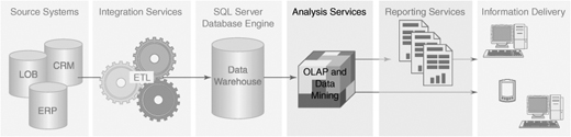
From an architectural point of view, the relational data warehouse is supplying the data storage and integrity, and the Integration Services packages are providing the data consolidation and cleansing. The Analysis Services database will extend the picture shown in Figure 5-1, providing the rich analytics and sheer performance that is required. Because we have defined views in the data warehouse for all facts and dimensions, the Analysis Services database can use these views as its source rather than accessing the physical data warehouse schema directly.
The users will connect to the Analysis Services cube using client tools such as Excel, which provides a drag-and-drop metaphor for easily accessing the information. Also, reporting tools such as Reporting Services can access the information in the cube, making it easier to publish the information to end users.
Although many people think of OLAP technology or cubes as restricted to being used for drilling down and pivoting through data, Analysis Services 2005 databases will generally remove the need for reporting directly from the relational data warehouse database. The reason for this is that Analysis Services uses an “attribute-based” model, meaning that all the columns in the underlying data source can be made available for analysis if required, instead of having to go back to the relational data for detail data.
Although you can use Analysis Services databases to add analytics to most data structures, the best solution to some calculation issues is to modify the underlying database. We make some changes to the fact views in the data warehouse to present information to Analysis Services in the way we need it for this solution.
The solution will deliver the following benefits to the client:
-
The solution will support the on-time delivery and profitability business initiatives by providing flexible analytical capabilities with the required subsecond response.
-
Allowing end users to directly access the information they need will reduce the pressure on IT to deliver new reports all the time and will free up valuable resources to work on other projects.
The data warehouse that we built in the previous two chapters already contains all the dimensions and fact tables that we need to support the business requirements, and most of the measures. In this section, we look at how the data model needs to be extended to more easily support building Analysis Services cubes.
The business requirements tell us that the users are interested in finding out how many (or what percentage) of shipments are on time, meaning that they were shipped on or before the due date. Because we already have ShipDateKey and DueDateKey columns that contain the relevant dates on the Shipments fact table, we should be able to calculate this without any problem.
In a relational reporting environment, we might add a where clause to our query that selected those records where one date was less than the other. It turns out that this approach is somewhat tricky to replicate in an OLAP environment, so we need another approach that can take advantage of the fact that cubes are very, very good at handling additive measures because of the power of precalculated aggregates.
We can start to solve the problem by realizing that each fact record is either “on time” or “not on time,” depending on the date values. If we have a Boolean value such as this in our data model, the best approach is to model it as a numeric field with a 0 or 1. For example, we could add an OnTime column to the fact table that contains 1 for an on-time delivery and 0 for a late delivery.
This works great for cubes, because then we can add a measure that simply sums the column to return the number or percentage of on-time deliveries. No matter how you slice the cube, whether you are looking at the total for the whole cube or just a specific customer’s shipments in the past week, the measure can simply sum the OnTime column.
TIP:
Transforming Logic into Additive Measures
Cubes are great at handling additive measures, so a common technique is to transform complex logic into a nice simple column. Logic that returns a true or false value is commonly expressed as a numeric column with a 0 or 1, or with a value such as a sales amount for some records and a 0 for other records.
This is especially true for logic that needs to be evaluated for every record at the detailed, fact-record level. Calculations that work well with totals (such as Profit Percentage defined as the total profit divided by the total sales) can more easily be handled with calculations in the cube itself.
Of course, because we have defined views over the fact and dimension tables and the views are going to be the source for the Analysis Services database, we don’t actually have to create a physical OnTime column. Instead, we can just add the calculation to the Shipments view using the following expression:
CASE WHEN ShipDateKey <= DueDateKey THEN 1 ELSE 0 END AS
OnTime
If you don’t have access to the views or tables in the source system, you can define the preceding SQL calculation in the Analysis Services database’s data source definition, but it is more flexible and easier to maintain if you define SQL expressions in the views. The performance penalty that some people associate with SQL date calculations isn’t particularly important in this case because the query will only be executed to load the data into the Analysis Services database.
An alternative approach to modeling this is to add a new On Time Category dimension that has two records, On Time and Late. This has the advantage that users could select a dimension member and restrict their analysis to only those shipments that fall into that category. Which of these options (or both) that you choose will depend on your users’ preferences, underlining again the benefits of prototyping and involving the users in design decisions that they will ultimately end up living with.
Another area that users will want to explore is the time periods for the shipments. For example, users need to know how many days late shipments were. They could perform some interesting analyses with this information, such as the average days late for a specific product or time period.
In a relational report, we could add an expression that calculates the number of days between the ShipDateKey and DueDateKey, which would give you the number of days late. This is another example of logic that needs the detail-level date keys to return a value, so we can add another calculated column to the view. Because we are trying to figure out how many days late the shipments are, and number of days happens to be a nice additive value, we can add an expression that returns the days between the two keys:
DATEDIFF(dd, DueDateKey, ShipDateKey) AS DaysLate
Actually, this expression turns out not to work so well because some shipments are early, so you will have negative DaysLate values that will tend to reduce the apparent lateness. This will require you going back to the users for clarification, but in the manufacturing example they don’t want to get credit for those shipments that happened to be early. (In fact, that might be another area they are interested in analyzing further because it has interesting business implications.) We need to adjust the expression so that shipments that are on time or early do not contribute to the Days Late value:
CASE WHEN (ShipDateKey < DueDateKey) THEN 0
ELSE DATEDIFF(dd, DueDateKey, ShipDateKey) END
AS DaysLate
We can handle the other business requirements in this area in the same way, such as calculating the number of days notice that we had by subtracting the due date from the order date and calculating the number of days it took to actually ship the product by subtracting the order date from the ship date.
If you add columns to your fact table that aren’t fully additive, such as Unit Price or Product Standard Cost, when you build your cube, you will start to realize that they don’t work very well. A cube generally sums up the values for the records that the user is looking at, based on their dimension selections. Analysis Services 2005 has some other ways of aggregating numbers beyond a simple sum such as Max or Min, and even supports some advanced scenarios for dealing with data that behaves strangely over time; by and large, however, most measures are summed.
Unit Price doesn’t work when you sum it. Although the Quantity Shipped sums very nicely under all conditions, the sum of the Unit Price for all shipments last year is meaningless. That is why the data model instead has an Extended Amount column, which contains the quantity multiplied by the unit price for the product. You can add up all the extended amounts for all shipments and come up with a useful number.
On the other hand, if the users needed to see the average unit price for the shipments, you can easily add a calculated measure to the cube that divides the total Extended Amount by the total Quantity, which is probably what the users wanted all along.
In contrast to a relational database, which is solely designed as a reliable data storage engine, you can think of an Analysis Services database as a rich semantic layer that provides information to users in the way they like to think about it, and which also loads data into a cache with some precalculated summaries to increase performance.
We start by using the BI Development Studio to create a new Analysis Services project. This will create a new local folder on your development machine that will contain the definitions for the Analysis Services objects that we will be creating. Later when we have finished designing the objects, we can deploy the project to a server that is running Analysis Services to create the cube and allow users to access the information.
You will notice that this is a different approach from working with normal relational databases. So far, when we have used the SQL Server Management Studio for tasks such as defining the data warehouse database, any modifications that we made to objects such as tables or indexes were immediately updated to the live database when we clicked the Save button.
All Analysis Services databases have one or more data sources that contain the information that will be loaded into the cubes. In our example, the source will be the manufacturing data warehouse database. The first step for creating an Analysis Services project is to add a data source and specify the type of database and connection information, using the same techniques we used for Integration Services projects in the previous chapter.
Most source databases contain a large number of tables and views. You can select the parts of the source database that will be used for analysis by defining a logical view of the database called a data source view (DSV), so we will be focusing this logical view on the dimension and fact views that we created when we set up the database. The DSV can also be used to define relationships between objects and to implement business logic by adding calculated columns to the logical view.
The DSV acts as an abstraction layer over the source system and can prove useful when you are building cubes over legacy data sources where you don’t have access to add simplifying views over the normalized underlying schema. When using data warehouses as the source, it is usually better to add any required business logic or calculated columns into the underlying views rather than using the DSV. As discussed in the “Data Modeling” section, we can add calculated columns to the underlying views in the database. These views can then be managed along with their corresponding tables and can be made available for other applications, too.
After we have added all the dimension and fact views to the DSV, we need to create the relationships between them. If we were using physical tables rather than views, the wizard that created the DSV could detect these relationships based on the primary key and any referential integrity constraints, but this doesn’t work for views, so we need to create the relationships manually.
The simplest approach is to arrange the dimension tables roughly around the fact table, as shown in Figure 5-2, and then drag each key column from the fact table to the corresponding dimension table primary key column. We also need to create the relationships for any snowflake dimensions such as Product. Similar to the fact columns, you drag the foreign key to the primary key (such as dragging the ProductCategoryKey column from Product Subcategory to Product Category).
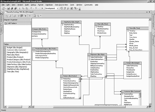
For dimensions such as Customer, there may be multiple relationships with the fact table. You can simply repeat the drag-and-drop process for each column on the fact table, such as ShippingCustomerKey and BillingCustomerKey. This is referred to as a “role playing dimension” in SQL Server Books Online.
TIP:
Dealing with Multiple Date Relationships
Fact tables frequently contain multiple date columns, which are often used to calculate values such as the total time taken to move from one state to another. When you are defining relationships in the DSV, you may decide to create relationships between the Time dimension and the fact table for each of the date columns. This makes sense as long as users are going to expect to be able to analyze the information by each of the different dates. So, when the users are looking for year-to-date sales, they would need to decide which kind of date analysis they would use, such as by order date or ship date.
For the Time dimension in the Manufacturing database, we will create relationships for the ShipDateKey, OrderDateKey, and DueDateKey columns on the Shipments fact table. This decision (like many decisions in BI) will make some things easier and others harder. If we had defined a single relationship with the ShipDateKey column on the Shipments fact table, this would have made things simpler for the user. There would be no ambiguity about which Time dimension to pick, but users would not be able to perform certain analyses such as the number of orders placed last month versus the number of orders shipped.
Building the Initial Cube
Now that the logical data model has been defined in the DSV, we can create a cube. BI Development Studio includes a wizard that will analyze the relationships that you have defined, as well as the actual data in the tables; the wizard usually produces a pretty good first pass for a cube design. The wizard makes suggestions for which tables are probably facts and which are probably dimensions, and also looks at the data in your dimension columns to try and come up with some reasonable attributes and hierarchies where possible.
A single cube can contain many different fact tables with different granularities and different subsets of dimensions. Each fact table that you include in a cube becomes a measure group, with a corresponding set of measures based on the numeric fact columns. This allows users to easily compare information from different fact tables, such as comparing Actual Revenue from a Sales measure group with Planned Revenue from a Budget measure group. This may trip you up if you are familiar with other BI technologies that had one separate cube per fact table—in Analysis Services 2005, the most common approach is to have only one cube in the database with multiple measure groups.
QUICK START: Creating an Analysis Services Cube
Before you can create a cube, you need to use BI Development Studio to create a new BI project with a data source and DSV. You also need to use the DSV to define the relationships between the tables:
-
Select New Cube from the Project menu, and click Next to skip over the welcome screen.
-
We will be using the wizard to recommend the cube structure, so leave the Auto Build checked and select Create attributes and hierarchies. Click Next.
-
Click Next again to select the Manufacturing data source.
-
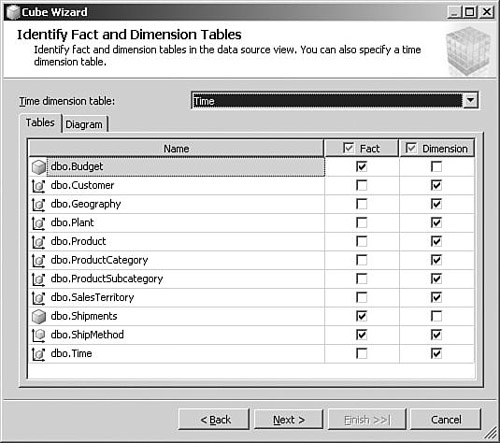
The wizard uses the relationships you have defined in the DSV to identify fact and dimension tables. Click Next to see the results (see Figure 5-3).
-
5. Make sure to select the Time dimension table from the drop-down list at the top of the page. You can now review the list of tables and check which were identified as facts or dimensions. If there are any strange selections, you can either fix them manually or return to the DSV to define relationships correctly. Click Next.
-
6. Because you selected a Time dimension in the previous step, you now need to let the wizard know the contents of the columns in the table (that is, which column contains the Year, which contains the Month, and so on). Make sure to select the TimeKey column as the Date selection. Click Next.
-
7. You can use the Select Measures step to rename measures or measure groups and to select any numeric columns that the wizard identified that are not actually measures. A good example of this is the Invoice Line Number and Revision Numbers column, which need to be unchecked because they are not measures. Click Next.
-
8. The wizard now reads the data in the dimension tables to see whether it can detect any hierarchies. Click Next to review the hierarchies that the wizard detected, along with the attributes found. You can use this step to uncheck any attributes or hierarchies that you don’t want to include in the cube. Click Next.
-
9. Give the cube a name that will be meaningful to users, such as Manufacturing. You may be tempted to use the name of a fact table here, but remember that later versions of your cube may include other business areas, so it is better to be quite general. Click Finish to create the cube and dimensions.
You may have noticed that the Ship Method table was identified as both a dimension and a fact. This is because there are numeric or money columns on the dimension table, and the wizard is including the table as a possible fact because the users might want to include those columns as measures in a query. In addition to having a Ship Method dimension, the cube will include the numeric measures from the Ship Method table as part of a separate Ship Method measure group.
TIP:
Why the Wizard Sometimes Identifies Dimensions as Facts
When using the Cube Wizard, you will often get to the step that shows which tables were identified as facts or dimensions and see that one of your dimension tables is incorrectly showing up as a fact. This is often due to a missing relationship or a relationship defined in the wrong direction in the DSV, and can usually be fixed by canceling the wizard, returning to the DSV to define the relationship, and then rerunning the wizard.
When you select a Time dimension in the Cube Wizard, you are prompted to specify the types of columns in the table. For example, you can select calendar year, month and day columns, as well as the equivalent columns that contain fiscal or manufacturing calendar information. The wizard uses the types that you select to apply special logic for time dimensions such as creating sensible hierarchies, and calculation formulas that you may add to the cube, such as year-to-date values, also use these types.
For elements such as years or months, Time dimension tables often have both descriptive columns containing the name of the period (such as FY 05 or Quarter 2), as well as a key column that identifies the period. This key column may be unique, such as a datetime column storing the first day of the period as the key (for example, 1/1/2006 for the first quarter of 2006). Alternatively, the key column may be a repeating number, such as using the numeric index of the period (for example, 3 for March).
When designing the Time dimension table, it is better to use the first approach (that is, create unique keys for periods), and then select these unique keys when specifying Time dimension periods in the wizard. Using the unique keys rather than the descriptions (such as selecting Year rather than Year_Name) will result in more efficient storage and avoid any problems with hierarchies that may be caused by nonunique keys, such as strange-looking hierarchies with members in the wrong places.
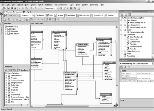
When the wizard has finished creating the cube, it will be opened up in the cube designer. You can use the Cube Structure tab shown in Figure 5-4 to view the dimensions and measures in the cube, and to add or remove new measures and dimensions. Before we start changing the structure of the cube, however, we should probably take a look at how the cube would look when a user browses it.
If you click the Browser tab after creating a cube, you get an error message that “Either the user does not have access to the database, or the database does not exist.” The problem is that although Visual Studio has created the files on your local PC that describe the definition of the cube and dimensions, we have not yet deployed these definitions to the server or loaded data into the objects. If you have a background with relational databases, you can think of our progress so far as similar to having used a fancy designer to generate a bunch of CREATE TABLE SQL statements, but not having executed them on the database server to create the tables, or loaded any data into them.
You can fix this problem by selecting Process from the Database menu. Visual Studio will detect that the definitions that you have created on your development PC differ from the definitions on the server and prompt you to build and deploy the project to the server first. When this deployment has been completed, the server will contain the same cube and dimension definitions that you designed locally, but they will still not contain any data. After the definitions have been deployed, you are prompted to process the database. This executes queries against the source database tables to load the cube and dimensions with data. Note that this might take a while when you have large volumes of data.
You can change to which server the database is deployed by choosing Properties from the Project menu and changing the target server.
The cube browser in BI Development Studio is intended to show developers how the cube will look when users browse the information. Of course, this assumes that the users have access to a BI application that supports the new features in SQL Server 2005, such as measure groups and attributes. If not, their experience may be very different, and you should test your cube design in the applications that they will ultimately use.
To use the browser, just drag and drop the measures that you want to analyze on to the center of the display, and then drag any hierarchies or attributes on to the columns and rows (see Figure 5-5). You can start to see how some of the decisions that the wizard makes show up in the browser, such as names of measures and attributes, and how hierarchies are structured. After building the initial cube, you will probably want to spend some time trying out different combinations and taking note of aspects that you would like to change.
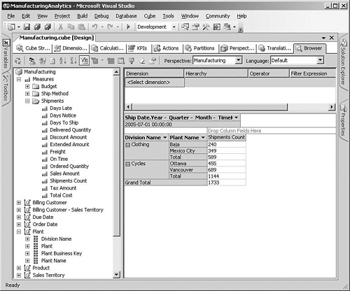
For example, you may notice that the wizard has not created any hierarchies for the Plant dimension, even though it would be useful for users to be able to drill down through divisions to plants. Because Analysis Services 2005 is attribute based, users could actually build this hierarchy dynamically at runtime by simply dropping the Division Name on to the rows, followed by the Plant Name. Still, it is usually helpful for users to see some prebuilt hierarchies, so we will go ahead and add some in the next section.
If you are building a cube that doesn’t have much data in the fact table yet, you might have difficulty figuring out how your attributes and hierarchies will look because the browser by default only displays rows and columns that actually have data. If you want to include the rows with no associated fact data, select Show Empty Cells from the Cube menu.
After we spend some time browsing through the data in the Manufacturing cube, we can see that we need to change a number of areas. This is where developing BI solutions gets interesting, because there are probably no clear requirements that you can turn to that say things like “the users would probably prefer to have a Divisions hierarchy to pick from rather than selecting two or three plant attributes manually.” There is a lot to be said for an iterative approach to developing cubes, where you build prototypes and show them to users for feedback, and then release versions of the cube to allow the users time to explore the system and give more feedback.
Because many dimension tables contain a lot of fields that are not particularly useful for users, you should exercise some care about which attributes you create rather than just creating an attribute for every field. Too many attributes can be confusing to users, and for very large dimensions, it may impact query performance because each attribute expands the total size of the cube.
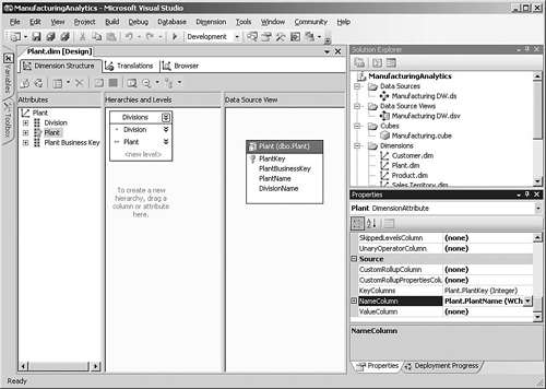
When the Plant dimension was created, the wizard created separate Plant Name and Division Name attributes. There is also a special attribute called Plant based on the PlantKey column. Each dimension has one attribute like this that has its Usage property set to Key, usually based on the surrogate key, which uniquely identifies a dimension record but doesn’t actually contain any information that the user would be interested in seeing. If a user includes the Plant attribute in the browser, the user will see meaningless integer values.
What we can do to fix this is to change the Plant attribute so that the plant name is displayed rather than the surrogate key. This can be accomplished by clicking the Plant attribute in the dimension designer, going to the NameColumn property in the Properties window, and selecting the Plant Name column. This means that having a separate attribute for Plant Name is now redundant, so we can remove it by selecting the attribute and clicking the delete button.
Also, now we have one attribute called Plant and another called Division Name, which is somewhat inconsistent, so it’s probably a good idea to change the attribute name to Division because you are not restricted to using the original source column name for an attribute (see Figure 5-6).
A hierarchy is a way to organize related attributes, providing a handy way for users to navigate the information by drilling down through one or more levels. Although users can define their own drilldown paths by dragging separate related attributes onto the browser, providing a sensible set of hierarchies for each dimension will help them to get started with common analyses.
The next change we make for the Manufacturing cube is to add a hierarchy to the Plant dimension that drills down through Division and Plant (see Figure 5-6). To set up our hierarchy, you can drag the Division attribute on the hierarchies and levels area of the dimension designer, and then drag the Plant name underneath it to create two levels. The name will default to Hierarchy, but this can be changed by right-clicking the new hierarchy and choosing Rename to change the name to something more meaningful.
Usually when you define a hierarchy, the bottom level contains the key attribute for the dimension (Plant, in this case) so that users can drill down to the most detailed data if they want to; this is not mandatory, however, and you can create hierarchies where the lowest level is actually a summary of dimension records.
Another area of the dimension that you might sometimes want to change is the name of the All level. When you include a hierarchy as a filter in the cube browser, the default selection is the top of the hierarchy, which includes all the data in the dimension. The name that displays for this special level can be changed for each hierarchy using the AllMemberName property of the hierarchy, such as All Divisions for the hierarchy we just created. You could make a similar change to the dimension’s AttributeAllMemberName property, which affects the name used when any simple attribute is used as a filter.
One of the most important steps you need to take when working with dimensions is to correctly define the relationships between attributes. For example, in a typical Geographic dimension, city is related to state, and state is related to country. These relationships are used by Analysis Services to figure out which aggregates would be useful, so they can have a big impact on the performance of your cube and also affect the size of your dimensions in memory.
If you look at the structure of the Time dimension that the wizard has created, you can see that we can clean up a few areas. When we set up the Time dimension in the Cube Wizard, we specified the key columns such as Year and Quarter rather than Year_Name or Quarter_Name, so we also need to change the NameColumn property for each of the attributes to point to the corresponding text column containing the name of the period. We can also rename the hierarchies and some of the attribute names.
If you expand the key attribute in the Dimension Structure tab, you will notice that the wizard created a relationship between the key attribute and every other attribute. The reason is that each attribute needs to be related to the key in some way, and it is technically true that every attribute can be uniquely determined by the key. When you think about how calendars actually work, however, you can probably see that there are other potential ways of defining these relationships. Each month belongs to one quarter, and each quarter belongs to a single year.
Because strong relationships exist between the time period levels, we should define the attribute relationships accordingly so that each child attribute has a relationship with its parent. Starting with the regular calendar periods of Year-Quarter-Month-Date, we can expand each of the attributes in the attributes pane on the left, and then drag the Year attribute onto the <new attribute relationship> marker under the Quarter attribute, and drag the Quarter attribute onto Month. The final level of relationships between Month and Date is already defined by default, so we don’t need to create this, but we do need to delete the existing Year and Quarter relationships under the Date attribute because these have been defined in a different way (see Figure 5-7).
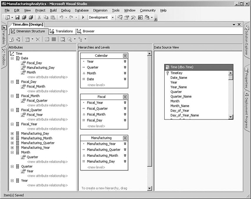
The same approach applies to the Fiscal and Manufacturing attributes because they also have strong relationships, so we can repeat the process of relating Fiscal_Year to Fiscal_Quarter, Fiscal_Quarter to Fiscal_Month, and Fiscal_Month to Fiscal_Day. However, every attribute needs to be related in some way to the dimension key, whether directly like Month or indirectly like Year. So, we also need to create a relationship between Fiscal_Day and Date so that all the fiscal attributes also have a relationship with the key.
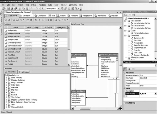
Now that we have the dimensions looking more or less the way we want them, we can turn to setting up the cube itself. The Cube Structure tab in the cube designer shows the measures and measure groups that have been defined, as well as a diagram that shows the underlying parts of the data source that make up the cube.
One of the areas that you probably noted when browsing the cube was that the numeric formats of the measures didn’t really match up with how users would want to see the information. For example, currency measures are shown with many decimal positions. You can change the display format by selecting a measure in the Cube Structure tab and modifying the FormatString property. The formats that you can specify are based on the Visual Basic syntax, which basically consists of a set of special named formats such as Percent or Currency, as well as characters that you can use to build user-defined formats.
If you have a lot of measures, changing the formats one at a time is painful, and the standard view of measures doesn’t allow you to select more than one measure at a time. A feature can help with this, as shown in Figure 5-8: Select Show Measures In Grid from the Cube menu, and you can then select multiple measures at a time and set all their formats simultaneously.
When the wizard was creating the cube, it looked at the relationships that you had defined between the fact and dimension tables in the DSV to determine how to add the dimensions to the cube. You can adjust the results using the Dimension Usage tab in the cube designer, which shows the grain of the different measure groups (see Figure 5-9).
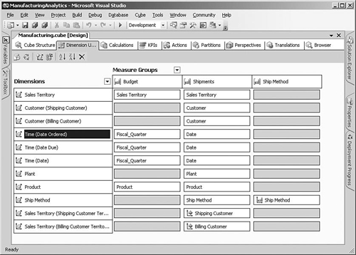
We need to modify a few things to get the cube to work the way we want. As you can see, a dimension such as Time or Sales Territory can be used multiple times in a single cube. The names that are shown to the user for these role-playing dimensions are based on the column names from the fact table. For example, the names that were created for the Time dimension are Due Date, Ship Date, and Order Date. You can modify these names by clicking the dimension on the left side of the Dimension Usage tab and then changing the Name property.
Usually, the order date is used as the standard way of analyzing a date, so we can name this relationship Date and rename the others to Date Due and Date Shipped so that they are listed together in the users’ tools.
Many of the key measures that are part of our manufacturing solution are just pulled directly from the fact table, but a lot of the really interesting information that the users need is derived from the basic data. Cubes can contain calculated measures that take data from the physical measures and apply complex logic. These calculated measures are computed at query time and do not take up any disk space; and because they are based on the Multidimensional Expressions (MDX) language, you can create sophisticated metrics if necessary.
One of the major business requirements is to analyze how the company is doing when it comes to delivering shipments on time. We have already added some physical measures such as On Time Count that can help with this, but we need to add more to the cube to really allow the users to make decisions. For example, it’s probably more important to be able to see the percentage of shipments that were on time rather than just a count.
To add the calculated measure, switch to the Calculations tab and click the New Calculated Member button (see Figure 5-10). The formula for this measure is simply the number of shipments that were on time, divided by the total number of shipments:
[Measures].[On Time Count]/[Measures].[Shipments Count]
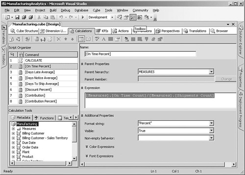
The major rule that you need to follow when naming calculated measures is that if you include spaces in the name, you have to surround the whole name with square brackets, such as [On Time Percent]. Because the name inside the brackets will be shown in the users’ analytical tools, it’s a good idea to use spaces and try to make the name as meaningful as possible. This may be counterintuitive for database designers who are used to avoiding spaces in names, but it is important to remember that the names in an Analysis Services cube are shown to users and need to make sense to them.
If you tried to use the Days Late or similar measures that we discussed in the “Data Model” section in a query, you will probably have realized that they are not useful at the moment because they just give the total number of days late for whatever filters you specify. A much more useful measure is the average number of days late for whatever the user has selected, whether that is, for example, a certain type of product or a date range such as the past three months.
The formula to express the average days late is to divide the total number of days late by the number of shipments in question:
[Measures].[Days Late]/[Measures].[Shipments Count]
Because the three physical measures (Days Late, Days Notice, and Days To Ship) aren’t really useful, we can switch back to the Cube Structure tab and change the Visible property of each of the three measures to False after we have created the equivalent average calculations. This is a common approach for measures that need to be in the cube to support calculations, but should not be shown to users.
We have some helpful measures such as Total Cost and Discount Amount in the cube, but the other business requirement that we need to support more fully is profitability analysis. Although profitability calculations are not particularly complex, it is much better to define them centrally in the cube instead of requiring users to build them in their client tool or add them to reports.
Percentages are often a useful way to understand information, such as adding a Discount Percentage measure that expresses the discount as a percentage of the total sales amount. Users could then select groups of customers to see what kinds of discounts they have been offered, or look at product categories to see which products are being discounted.
We can also add a Contribution measure that shows the profit achieved after deducting costs and discounts. Because it will probably be useful to also see this number as a percentage, we can add another measure that divides the new Contribution measure that we just created by the total sales amount:
[Measures].[Contribution]/[Measures].[Sales Amount]
You can use the Browser tab of the cube to test the calculated measures that you have defined. It’s a good idea to try different filters and combinations of dimensions on the rows and columns to make sure that your new measures make sense in all the circumstances that the user will see them. Because adding a calculation is a change to the structure of the cube, you need to deploy the solution again and click the Reconnect button in the cube browser to make the new measures show up.
The first thing you will notice is that your new measures are not grouped under the existing measure groups such as Shipments or Budget, but are at the bottom of the list. Because the users probably don’t care which measures are calculations and which are physical measures, you should go back to the Calculations tab and select Calculation Properties from the Cube menu and specify an associated measure group such as Shipments for each of the calculations.
Several columns on the fact table contain potentially useful information that we cannot define as measures because they have no meaning when they are aggregated. For example, if users are looking at all the shipments for the past year, there is no point in showing them the total or average of all the thousands of Carrier Tracking Numbers or Customer PO Numbers.
This kind of column is often referred to as a degenerate dimension, because you can think of it as a dimension with only a key (like Order Number) and no descriptive attributes. Analysis Services 2005 instead uses the term fact dimension, meaning a dimension that is based on a fact table.
Figure 5-11 shows how a user can see the invoice and carrier tracking numbers for a set of shipments by selecting attributes from the Shipment Details dimension that we just created.

The last step before we can deploy our solution is to figure out which users will need to have access to the database and whether they will need to see all the information or just parts of it. You can develop sophisticated security schemes by adding roles to your Analysis Services project, by selecting New Role from the Database menu.
Each role defines which cubes and dimensions users will have access to, and can even restrict the data that they will see (for example, limiting the Sales Territory dimension to show only North American territories for U.S. sales reps). Dimensions or measures with potentially sensitive information can be turned off completely for some groups of users.
After the role has been defined, you can set up the membership by adding Windows groups or specific user accounts to the role. You can test that the role is working the way you intended using the cube browser, by clicking the Change User button on the left of the toolbar and selecting the role.
We have so far been using the BI Development Studio to develop the project and deploy it to the server. After the database has been deployed, the emphasis switches from developing a solution to managing the deployed database, and you will be using the same SQL Server Management Studio that you used to manage SQL Server databases.
To connect to an Analysis Services database from SQL Server Management Studio, select Connect Object Explorer from the File menu, choose Analysis Services as the server type, and select the server name before clicking the Connect button.
As you have seen while developing the cube in the “Technical Solution” section, you can deploy an Analysis Services database directly from within the BI Development Studio. This proves to be very useful during the development phase; when you need to move the database to a test or production environment, however, a more structured approach is required.
Analysis Services 2005 includes a Deployment Wizard that can either interactively deploy the database to a specified server or create a deployment script that can then be executed on the target server using SQL Server Management Studio. You can access the Deployment Wizard from the Start menu, under the Microsoft SQL Server 2005, Analysis Services folder (see Figure 5-12). The source file that the wizard uses is a file with an .asdatabase extension that is created in your project’s bin folder when you build the project in BI Development Studio.
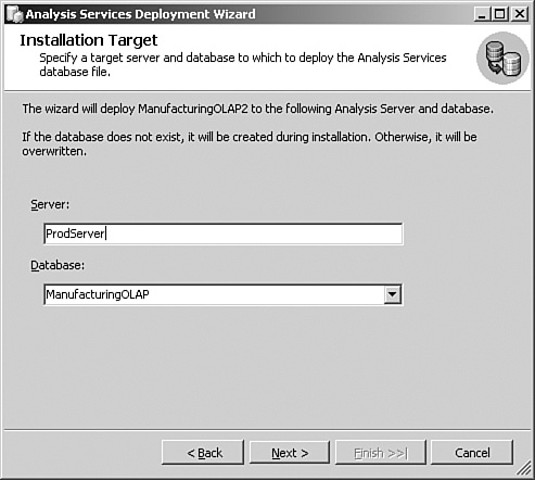
The wizard also gives you control over the configuration settings for your Analysis Services database. For example, if you are deploying to a production server that uses a different database from development, you can specify a different data source connection string and impersonation setting for the deployment. You can also choose not to overwrite any settings such as role members or connection strings (in case these have been modified on the target server by the system administrator).
That takes care of getting your new database definitions on to the target server, but what about initially loading the data? The wizard also enables you to specify that objects must be processed after they have been deployed, including an option to use a single transaction for processing objects and roll back all changes if any errors are encountered.
Analysis Services server administrators can perform any task on the server including creating or deleting databases and other objects, administering roles and user permissions, and can also read all the information in all the databases on the server. By default, all members of the server’s Administrators group are Analysis Services server administrators, and you can also grant additional groups or individual users server administration rights by right-clicking the server in SQL Server Management Studio, selecting Properties, and then adding them to the server role in the Security section.
You can change the default behavior that grants local administrators full Analysis Services administration rights by changing the BuiltInAdminsAreServerAdmins setting to False, but this is not a worthwhile exercise because this setting is stored in the configuration file for Analysis Services, which local administrators would probably have access to anyway. Also, because you can actually have multiple Analysis Services instances on a single server, technically speaking a server administrator is actually an “instance administrator” because the permission is granted for an instance, not necessarily the whole server.
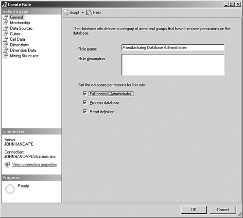
If you have an environment where you want to grant administrative privileges only to specific Analysis Services databases rather than all of them, you can create a role in a relevant database and select the Full Control (Administrator) permission, as shown in Figure 5-13. The groups or specific users who need to administer that database can then be added to the role. Database administrators can perform tasks such as processing the database or adding users to roles.
If you add roles to a database using SQL Server Management Studio, you need to be aware that they will get overwritten if you redeploy the project from BI Development Studio. You must either add the roles to the project in BI Development Studio so that they always exist, or deploy the project using the Deployment Wizard with either the “Deploy roles and retain members” or the “Retain roles and members” option selected. If you select “Deploy roles and members” in the wizard, any roles that you manually created using SQL Server Management Studio are removed.
Every BI solution that we have ever delivered has required some enhancements, usually soon after deployment. The reason for this is intrinsic to the way people use BI applications, in that every time you show them some interesting information, they immediately come up with a specific aspect that they would like more detail on.
You can use the BI Development Studio to make changes to the project files and redeploy them to production using the method described in the “Deployment” section, but it is a great idea to start using a source code control system for these files. In addition to making it easier to work in a team environment, source control enables you to keep track of the versions of the solution that you have created.
At some point, you are probably also going to have to make changes to the underlying source database, such as adding new columns or new fact and dimension tables. Because we have recommended that you build the Analysis Services databases from views rather than directly on the tables, this will probably provide you with some protection because you can make sure that the same schema is presented if required.
However, if you want to include these new database objects in your Analysis Services project, you must update the database views and then open the relevant DSV in BI Development Studio and choose Refresh from the Data Source View menu. The Refresh feature has a nice user interface that shows you what (if anything) has been changed in the source objects, and then fixes up the DSV to match.
One important caveat applies, however: Any objects based on the changed database object will not automatically be fixed, and you need to manually address these. For example, if you changed the name for a database column, the corresponding attribute will still have the old column name and must be updated manually.
The major operations tasks that you need to perform for Analysis Services are processing the databases and making backups.
As you have seen when using the BI Development Studio to create a cube, after Analysis Services objects have been deployed to a server, they need to be processed before users can access them. This kind of processing is known as full processing, and it will usually take some time in production systems because all the data for dimensions and facts is read from the source systems and then used to create the Analysis Services databases.
Full processing must be performed whenever you have changed the database definition in certain ways, such as adding an attribute hierarchy. In most cases, however, you only really need to load the new data for the period, such as changes to the dimension records or additional fact rows. For dimensions, you can select the Process Update option to read all the dimension records and create any new members, or update existing ones when they have changed.
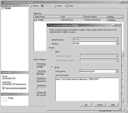
Measure groups are a bit more complex because you usually only want to add the new records from the fact table, so you need to supply a way to enable Analysis Services to identify those records. The Process Incremental setting shown in Figure 5-14 enables you to either select a separate table that contains the new records you want to load or to specify an SQL query that only returns the relevant records.
Because the Analysis Services processing usually needs to be synchronized with the ETL routines that load the data warehouse, a common approach is to add an Analysis Services Processing Task into the Integration Services packages for the load process.
If a disaster happens to your Analysis Services database, one way of recovering is to redeploy from the original project source code and then reprocess the database. So, a key part of your backup strategy is to always have an up-to-date backup of the solution files or the source control repository. However, reprocessing can be very time-consuming, so the usual approach is to make a backup of the Analysis Services database, too.
You can back up the database from SQL Server Management Studio by right-clicking the database and choosing Back Up. Figure 5-15 shows the options that you can specify. The backup process creates a single .abf file containing the metadata and data for your database, and this can optionally be compressed.
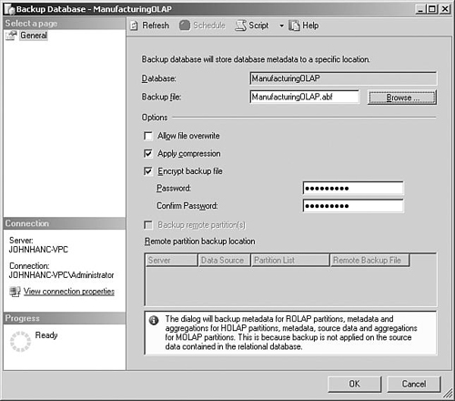
Because these databases often contain sensitive information, you can also specify a password that is used to encrypt the file. It is worth being careful with this password, however, because you will need it to restore the backup if necessary and the file cannot be decrypted if you lose the password.
If you need to recover the database, you can restore the backup by right-clicking the Databases folder in SQL Server Management Studio and selecting Restore.
The previous three chapters showed how to build the foundation of a complete BI solution, including a data warehouse, ETL process, and Analysis Services database. These are really the basic building blocks that we use as the basis for the rest of this book, which covers the other areas that you need to understand to start building valuable BI solutions. From now on, each chapter covers a specific solution for a single customer from end to end to demonstrate one specific aspect of BI in detail.
We have shown you in detail how to build a complete solution to a very small part of the total manufacturing picture: shipments. Real-world solutions could be extended into whole new business areas to analyze the manufacturing process itself, or the performance of the manufacturer’s suppliers. Inventory management and optimizing the balances of products on hand is another area that could provide significant business value. Whatever area that is chosen should lead to another small iteration of our BI development process, with carefully defined objectives leading to a new release.
We have looked at how to build a cube in this chapter, but we glossed over how users would access the information by simply referring to client tools such as Excel. A complete BI solution must supply information to users in whatever ways are most suitable for them, including Excel or other “slice-and-dice” client tools, but also other mechanisms such as web-based reporting or dashboards that show summary information and support drilldown for more details. Chapter 9, “Scorecards,” describes the approach to provide complete access to the information in your databases.
In this chapter, we used BI Development Studio in project mode, meaning that we worked on a set of project files that were stored on the developer’s workstation, and then we selected Deploy to update the definitions on the corresponding Analysis Services database on the server. BI Development Studio can also be used in online mode, by connecting directly to a live Analysis Services database.
You can access a database in online mode by selecting File, Open, Analysis Services Database, and then specifying the server and database name. Any changes that you make are immediately saved to the database. Be cautious not to mix project mode and online mode, however, because you could easily overwrite any changes you made in online mode by deploying a project.