
Our customer for this chapter is a major hospital that wants to optimize its allocation of resources, by being more aware of the immediate needs driven by the current patient profiles such as specialized staffing or perishable supplies.
A multidimensional database is used to manage hospital admissions and assist with patient diagnosis. Its purpose is to provide information to anticipate staffing requirements for the next shifts, determine medical-supply requirements, and provide early detection of elevated occurrences of contagious diseases or environmentally induced illnesses such as food poisoning. The data warehouse is populated overnight, but this does not give them sufficiently current information on which to base the day’s operational decisions. At the same time, they cannot afford to take the system offline for more frequent updates. To ensure quality patient care, they have often overestimated the resources required for each shift.
We will use Analysis Services proactive caching to enable real-enough time updates of our cubes. Proactive caching allows us to configure notifications of changes to the underlying relational table of a cube, and a maximum acceptable latency before the changes appear in the cube. We will isolate historical data and recent data from current data in separate partitions to reduce the amount of data that needs to be processed by the proactive cache. This will minimize the time between the arrival of new data and its availability to the user.
The database consists of a large amount of historical data as well as very current data. New data needs to be available in an OLAP database within 30 minutes of its arrival at the hospital. The OLAP database must be accessible to users continuously, even during updating. The medical staff needs to be able to track the current symptoms and medical requirements of new and existing patients and be able to anticipate the resources required by those patients over the next 24 hours.
A multidimensional database is required because of the large volume of data and multiple ways of analyzing the data. Our goal is to make new data visible as soon as possible after it arrives. One of the barriers to this is that with the MOLAP storage model, the data is only visible after the cube has been processed. We favor the MOLAP model because it is extremely an efficient way to store and retrieve cubes. It turns out we can trade some overhead for lower latency. The overhead arises from more frequent processing of the updated cube partitions, since processing is how data in the relational tables becomes available through the cube. By being smarter about what we reprocess, we hope to pay out as little as possible in overhead and in return receive a large reduction in latency.
For the Analysis Services database, we will use the Proactive Caching feature of Analysis Services to reduce the latency between the arrival of new data and the availability of the data to the user. For optimal access to the existing data, less-recent and historical data will be maintained as usual in MOLAP storage partitions. The new data will eventually make its way to one of these partitions or a newly created partition.
We will use the partitioning techniques discussed in the chapter on very large databases to limit the cube partitions that need to be processed. Ideally, only one very current partition needs to be processed.
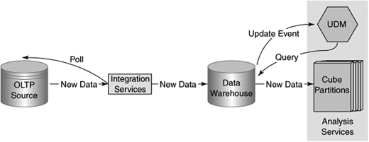
As shown in Figure 12-1, SQL Server Integration Services (SSIS) will receive data from external sources by periodic polling of the sources, apply the necessary transforms to make the data conform to our data model, and store the data in data warehouse tables. SQL Server will notify Analysis Services of the arrival of new data in the data warehouse. Analysis Services will process the new data when a lull in the arrival of new data occurs or when the latency constraints dictate that the data must be processed. You have total control of the definition of a “lull” and the maximum latency.
The hospital expects to reduce its operating costs by having the right number of staff with the right skills in attendance each shift. In addition, they expect to reduce waste of expensive supplies that have a short shelf life, kept on hand in quantities larger than usually necessary. They will now be able to analyze the current overall patient profile, bed utilization, and care-type requirements.
A day is a long time in the context of epidemics. With near real-time analysis, local health authorities will have much faster notice of epidemics, which will reduce the number of victims, reduce hospital visits, and thereby free space for the critically ill and reduce overall health-care spending.
Our facts in this example are patient diagnosis records generated throughout a patient’s hospital stay. These records are created by the medical staff as a patient’s condition changes. They are entered into the hospital’s patient monitoring application. The dimensions we are concerned with are Patient, Diagnosis, Date, Time, and Ward. The Patient dimension changes quickly; the other dimensions are static. This yields a data model like that shown in Figure 12-2.
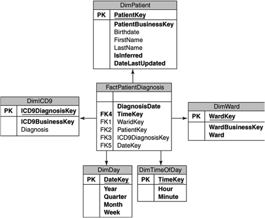
The main thing you need to do in your data model to accommodate real-time OLAP is to support partitioning and incremental loading. We are relying on a partitioning scheme to minimize the amount of reprocessing time, and we are relying on incremental loading to minimize the number of partitions affected during the loading of facts. We’ll use the DiagnosisDate column for both purposes. Our Patient dimension is also changing in real time, so we’ll need a column to track which patient records are new or updated. For that, we’ll use the DateLastUpdated. We can compare these column values against those in the source tables and load only the newer records.
In real-time applications, sometimes the facts arrive before new dimension members do. This would normally be classified as missing members. For example, unidentifiable patients might arrive at the hospital, and their symptoms and resource needs would be recorded, but we would not have a member for them in our patient dimension yet. We need to support inferred members, which we discussed in Chapter 7, “Data Quality.”
We’ll start by looking at what changes you need to make to your cube design for a real-time solution and work our way back to how we load data through Integration Services. Note that the basis of this solution, proactive caching, is only available in the Enterprise Edition of SQL Server 2005.
In all the other chapters, we have implicitly or explicitly urged you to use MOLAP storage for your cubes and dimensions because of MOLAP’s vastly superior performance over ROLAP. Remember that ROLAP mode simply references the relational database to answer queries and has no storage optimizations for the kinds of queries that are common in OLAP queries. However, you have to process a cube to load the relational data into MOLAP storage, and that step adds latency to making new data available to your users. With ROLAP storage, there is really no need to process the cube to make the data available, which is exactly what we are looking for in a real-time solution: present whatever data is available right now. So why not use ROLAP all the time? Because we can’t afford the query performance hit if we have a large amount of historical data and complex dimensions, and this is why we recommend MOLAP. Wait, this is where we started....
What we really want is the best of both worlds. MOLAP performance for all the existing data and low-latency ROLAP for newly arrived data. Fortunately, we can now design a system that approaches these characteristics. With Analysis Services 2005, you have the services of proactive caching available to you, which when combined with a good partitioning scheme integrates the performance benefits of MOLAP aggregations with the low latency of ROLAP.
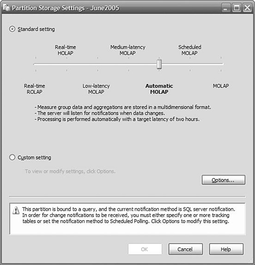
To enable proactive caching, open the designer for the cube. Select the Partitions tab. You probably have only one partition right now, but if you have more than one, choose the one that stores the “current” data. Click Storage Settings, be sure that the Standard Settings button is selected, and move the slider left, from MOLAP to Automatic MOLAP (see Figure 12-3). Save these settings. Congratulations, you’re done! Go browse your cube and note the value of one of the measures, add a row to your fact table, wait 10 seconds, and then refresh the display. The new data really is there, and you didn’t even have to process the cube.
Now that was too easy, you say, and there must be a catch. Well, there are some considerations, but no real catches. First, it’s important to understand how proactive caching really works, and then you will have a better idea of the reasons for these considerations, and why there are not any big catches.
Let’s take a closer look at what we just did with proactive caching. Proactive caching sits between the user and the data they are after. In a static situation where MOLAP storage is used, a request for data is satisfied by the cache, which obtains all the data from the MOLAP store. Simple enough. When new data arrives in the relational store, the MOLAP cache is out of sync with the relational store. What are our options for dealing with the next request for data?
We could simply continue to serve up data from the cache and in the background begin rebuilding the MOLAP store. The data would be out of date until the reprocessing was finished, but we would still be responding to requests quickly because we are using the cache. How stale the data becomes is a function of how long it takes to reprocess the data.
If we need to have the most up-to-date view of the data, we could have the cache immediately invalidated when new data is received. Now our only source of data is the relational database, which means we are in ROLAP mode. This is the effect you get if you choose real-time HOLAP for the partition storage settings. ROLAP can be extremely slow for some queries.
We could do something in between these two extremes. We could continue to use the cache for a while, but if processing took too long, we could then invalidate the cache and use ROLAP mode. If we can reprocess the data before the data is too stale, we avoid having to go to the poorer-performing ROLAP mode.
You can configure proactive caching so that you recognize and wait for the completion of a steady stream of input, and at the same time don’t exceed your maximum latency requirements. Consider the following scenario. When new data arrives in the data warehouse, the sooner we start processing it, the sooner it will be available. So, what’s holding us back from processing this data? Well, what happens if more data arrives soon after we started processing? We have to start again, and that means we have to throw away the cycles we just consumed. Remember that we are not processing just the new data, but all the data in the partition. This could be your entire set! If we wait just a little while to see whether any more data is going to arrive, we could process it all at the same time. But how long should you wait?
Suppose that a batch upload to the data warehouse is occurring. There will be little time between the arrival of each row, and we certainly wouldn’t want to be restarting the processing after each row. So why don’t we wait, say, ten seconds after a row arrives, and if nothing else arrives, then we can start processing. If another row does arrive, we start waiting for ten seconds again. The time we wait to see whether the activity has quieted down is called the silence interval. If no data arrives for the duration set by the silence interval, and there is new data, processing begins.
You can set the value of the silence interval to any value from zero upward. Ten seconds is common. (That’s why you had to wait 10 seconds before refreshing your browser when we first started looking at proactive caching.) If you set the silence interval to zero, processing starts immediately when data is received but might be interrupted by the arrival of more data. If you set it to a very large value, processing does not start at all until that time is up, and you might get excessively stale data. However, we do have a solution to the problem of false starts of the reprocessing task, and you can tune this to your situation. But what happens if data continues to trickle in?
If you have set the silence interval to ten seconds, on a bad day the data will arrive one row every nine seconds, and nothing will ever get processed because the silence interval criteria is never met. After a while, we need to be able to just say “enough!” and start processing. This is where the silence interval override value comes in. The silence interval override timer starts as soon as the first new data arrives after processing. Even if data trickles in just under the silence interval value, when the override period is exceeded, processing starts regardless of whether the silence interval requirement has been satisfied.
You set the silence interval override to a value that makes sense for your requirements (of course you would!). By that we mean if you have batch updates occurring every hour, and they take about 10 minutes, you might set the silence override interval to 20 minutes. This means that there will be sufficient time to complete a batch update before processing starts, and as soon as the batch is finished, the silence interval will likely kick in and start processing ten seconds after the batch completes. If you have an exceptionally long batch, or the trickle updates are still defeating the silence interval, processing starts anyway.
Okay, we are doing well. We have solved the problem of being so swamped with new data that it never gets processed. But what if processing takes too long? Our data will be too stale to meet our business requirements. In a worst-case scenario, we have data that is 20 minutes old (the silence override interval) plus the time it is going to take to process the partition.
So far, we have learned about optimizing when we reprocess an updated partition. We didn’t want to waste resources if we were just going to have to restart with the arrival of new data. However, the user is still being given data from the MOLAP cache, and the cache is getting staler the longer we wait for processing to finish. If you have a requirement to present users with data that meets an “age” requirement, your only choice is to abandon the cache at that age. When the cache is not being used for data, queries are satisfied directly from the relational database (that is, by using ROLAP mode). Performance might not be good, but at least the data will be fresh.
You control when the cache is dropped by setting a time for the drop outdated cache property. The timer for this starts as soon as the first new data arrives, just as it does for the silence interval override. If you cannot afford to have data more than one hour old, set this value to 60 minutes. This setting guarantees that regardless of the arrival of any volume of new data, or how long it takes to process it, the data delivered to a user will meet this “freshness” criteria. You can set this value anywhere from zero up. If you set it to zero, the cache is invalidated immediately, and new data is available immediately. This might put quite a load on the server because most queries will now be resolved using ROLAP mode. Unless there is a long quiet period, data trickling in may keep the cache invalid most of the time, and you have traded performance for very low latency.
In all the tuning parameters we have discussed, we were always confronted with the time required to reprocess a partition. If you have a lot of data, it’s going to take a while to process it. However, we’ve already processed most of it; why bother to process it again? It’s because the unit of processing is a partition, and so far we’ve only set up one partition containing all our data. Performance will deteriorate over time, depending on how much data is added over time.
What we want to do is to put as much of the “old” data as possible in a partition by itself and leave it alone. We don’t enable proactive caching for this partition, so it will not be reprocessed unless we manually initiate it. In another partition, we can put the most recent, or “current” data. We would enable proactive caching only on the “current” partition, which we expect to be substantially smaller and so require much less time to process.
We would merge the current partition into the historical partition when there’s enough data in it that performance is affected, and then we’d create a new “current” partition. Let’s take a look at how that would work in practice. For this example, we’ll assume that our historical and current partitions are split at June 1, 2005.
QUICK START: Setting Up Partitions for Proactive Caching
In this Quick Start, we configure proactive caching so that it meets our requirements for real-enough time updates of our cube. Start by creating another partition so that you have one for historical data and one for current data. You learned how to create partitions in Chapter 11, “Very Large Data Warehouses,” so we won’t repeat those steps here. The current partition shouldn’t be so large that the reprocessing time exceeds your requirements for making new data available to your users.
Open your Analysis Services project in BI Development Studio, and we’ll begin configuring the proactive cache settings.
-
On the Partitions tab of the cube designer, select your current partition.
-
Click Storage Settings, and set the slider to Automatic MOLAP.
-
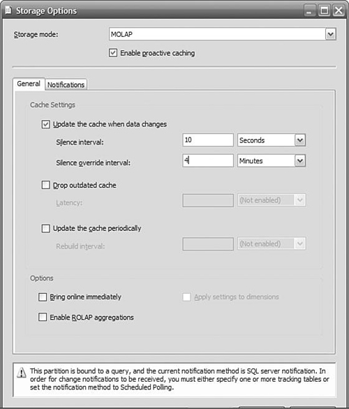
Click Options. Based on our measurements, our partition takes less than a minute to reprocess. We want a latency of less than five minutes, so we’ll set the Silence override interval to four minutes, as shown in Figure 12-4. This means the partition is guaranteed to start to be reprocessed within four minutes and will complete in less than five minutes, because we know from testing that the partition processing will complete in less than one additional minute.
-
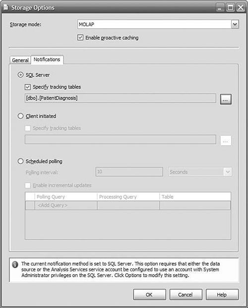
On the Notifications tab, Select SQL Server, and then check Specify tracking tables. We need to tell Analysis Services which table to monitor for changes because we specified a query instead of a table to define the data that will populate the partition. Click the ellipses (...) and select the fact table specified in your query where you defined the partition. Click OK to save the tables to be monitored, as shown in Figure 12-5, and then click OK and to save the Notification settings.
-
Click OK to complete the configuration of the proactive cache for the current partition.
At this point, we’d like to briefly expand on the options for notifications used by proactive caching to kick off the processing of a partition.
Proactive caching requires a notification to make it aware of new data. There are three basic methods available to you: notification “pushed” by SQL Server when a table changes, sending client-initiated XMLA message from a service or programmatically to Analysis Services, or polling at intervals to check for new data. You specify which method you want to use on the Notifications tab on the Storage Options dialog, as shown in Figure 12-5. As you saw earlier, you access the Storage Options dialog by clicking the Options button on the Partitions Storage Settings panel. But how do you choose which method is appropriate for your business requirements?
SQL Server Notification
SQL Server notification uses SQL Profiler to capture events that indicate a relevant table has been updated. This approach means that a notification is pushed to Analysis Services, which is much faster than Analysis Services polling for changes. Profiler does not guarantee that absolutely all update events will be detected, so it is possible that Analysis Services will not be notified, and your cube will not be as current as you expect. However, missed events usually result from heavy activity on the database, so it is likely that another event will trigger notification within a short time, and your cube will still be very current.
SQL Server notification only works with SQL Server 2005 databases, because it uses the SQL Server Profiler to detect table changes. If your data source is something other than SQL Server 2005, you cannot use this method to notify Analysis Services of a change.
Events are tracked through SQL Profiler using table names. Analysis Services can determine which table you are using in the partition and automatically monitor it. If you are using a view to populate the cube, you should specify the underlying tables that are actually being updated.
In the preceding example, we used SQL Server Notification.
Client-Initiated Notification
You can use the XMLA command NotifyTableChanged to alert Analysis Services of a table change. You use this notification method when your data source is not SQL Server and you need faster response time than you might get by polling. In the sample code shown next, an XMLA command is sent to the server MyAnalysisServer. Analysis Services will be notified that the PatientDiagnosis table has changed. This table is used by the OLAP database DiagnosisProfile, as specified by the DatabaseID. The table resides in a database referenced by the data source Health Tracking DW, specified by the DataSourceID.
Dim command As String =
"<NotifyTableChange
xmlns=""http://schemas.microsoft.com/analysisservices/2003/ engine"">" + _
"<Object>" + _
" <DatabaseID>DiagnosisProfile</DatabaseID>" + _
" <DataSourceID>Health Tracking DW</DataSourceID>" + _
"</Object>" + _
"<TableNotifications>" + _
" <TableNotification>" + _
" <DbSchemaName>dbo</DbSchemaName>" + _
"<DbTableName>PatientDiagnosis</DbTableName>"
+ _
" </TableNotification>" + _
"</TableNotifications>" + _
"</NotifyTableChange>"
Dim client As New Microsoft.AnalysisServices.
Xmla.XmlaClient
client.Connect("MyAnalysisServer")
client.Send(command, Nothing)
client.Disconnect()
Polling by Analysis Services
Polling is a method where a query is periodically sent to a data source by Analysis Services. It is useful when the data source is not SQL Server, and there is no application that can send an XMLA command to Analysis Services. Polling is usually less efficient and often means greater latency than other notification methods.
On the Notifications tab, you specify a query that is to be used to check for new data, and how often it is to be sent. This query must return a single value that can be compared against the last value returned. If the two differ, a change is assumed to have occurred, initiating the proactive cache timing sequence.
Just when you thought we had sorted out all the potential problems that could occur, some new fact records arrive in the data warehouse right in the middle of the cube processing—how do we avoid having an inconsistent picture? SQL Server 2005 has a useful new transaction isolation level called snapshot isolation, which uses row versioning to make sure that a transaction always reads the data that existed at the beginning of the transaction even if some updates have been committed since then.
To get Analysis Services processing to use snapshot isolation, you can change the Isolation setting on the Analysis Services data source from the default ReadCommitted to Snapshot. If you try this out, you will get a warning message that snapshot isolation won’t be used unless “MARS Connection” is enabled. You can turn on the MARS Connection property by editing the connection string in the Data Source Designer and then clicking the All button on the left to see all the advanced properties.
We’ve got Analysis Services reading from the data warehouse automatically. How do we get data from the source into the data warehouse in real time? Periodic polling of the source system is the easiest to implement. You can use SQL Agent to schedule an SSIS package to run periodically to import new data into the data warehouse. This works well when you can accept latency on the order of several minutes or more, which is acceptable in many applications. Avoid using polling when the latency requirement is measured in seconds, because of the cost of initiating the package every few seconds (even if there’s no new data).
In our example, we used polling because we can accept a latency of a few minutes. We created a job in SQL Server Agent with an SSIS package step that invoked our import package that loads the data warehouse. We set a schedule for this job that specifies a recurring execution every two minutes. When setting this time for your schedule, consider how long it takes to reprocess the current partition and either reduce the frequency of execution if the processing takes a good part of the two minutes or reduce the time window on the current partition so the processing time will go down.
You can initiate the importing of the data in other ways without polling if you have some control over the application that creates the data.
A message queue is a guaranteed delivery mechanism for sending data and messages between applications. The applications do not need to be on the same machine but, of course, do need some connectivity and authentication. MSMQ (Microsoft Message Queue) is a service that provides these features and is part of Windows Server.
You can use an MSMQ task in an SSIS control flow to listen for messages indicating that new data is ready, and then launch the data flow task to begin the data import.
Windows Management Instrumentation (WMI) monitors the entire system for certain events, such as file creation. You can use a WMI task in SSIS to wait for an event and then proceed to the data flow task when the event occurs. For example, your data source application might push a flat file to a directory that you monitor with WMI. When the file is dropped in the directory, your package detects this and begins the process of loading the data.
As we have described, the changes you need to make to enable real-time BI mostly relate to Analysis Services partition settings and Integration Services packages. The management of a real-time solution does not differ much from that of standard BI solutions, except that you need to pay careful attention to the complete process of handling new data. (Because there is no overnight processing window to give you time to smooth out any mistakes, users will be aware of any problems right away.)
Operation of a real-time OLAP database does not differ much from a regular OLAP database. You have the additional task of creating new partitions and merging old partitions.
In a real-time application, data usually trickles into the relational database on a continuous basis. There is no batch loaded at regular intervals. This means you must use the Full recovery model and back up the transaction log files to protect your database. You only need to back up the partitions that are read-write, which should just be the most recent partition.
Unlike a relational database with partitions, for Analysis Services you need to back up the entire cube each time. You may have expected to get away with only backing up the current partition, but you can’t because you cannot select which partitions to back up.
Although you can technically delete the relational tables underlying the partitions after the data has been loaded into Analysis Services, you should not do this. Partitions set to use proactive caching may revert to ROLAP mode depending on the settings and require the relational tables. More important, if you ever need to reprocess or rebuild the partitions, you must have the relational data. So, be sure that the data sources are formally backed up and are accessible to you.
Remember why we created partitions in the first place: so we wouldn’t have to reprocess more data than we had to. Therefore, we created a partition for history and another for the current month. We only reprocess the partition for the current month. In a perfect world, June data arrives in June, and July data arrives in July. However, this is not our experience. Data is delayed, or post-dated. It arrives out of sequence. Because of the reality of our business, we cannot simply close off the previous month and open the current month’s partition to updates.
Depending on your business rules, you might need to keep monthly partitions open for two or three months, and the current month’s partition must be open to all future dates. To maintain your partitions, you create enough “current” partitions to accommodate the latest data that could arrive out of sequence. If that’s 90 days, for example, you want three monthly partitions. Each partition will have a definite start and end date specified in the query to restrict the rows. The exception is the last partition, which does not restrict the end date of the fact rows.
When you create a new partition, you will likely retire an earlier partition by merging it with the historical partition.
After merging a number of current partitions into the historical partition, you need to reprocess the historical partition to improve the aggregations and efficiency of their organization. You should do this during a maintenance period due to the resource consumption of the operation. You need to monitor the performance of the server to determine how frequently this needs to be done.
With real-time data, you have the opportunity to do some interesting just-in-time analysis. Credit card companies look for spending that doesn’t conform to your usual patterns. In our health-care example, we could use data mining to understand the normal patterns of initial diagnosis at an emergency ward and look for deviations that might provide an early indication of the start of an epidemic or an outbreak of local food poisoning.
In a real-time application, the source data constantly changes. If you need to have a time-consistent view of the data loaded into the data warehouse, you can use snapshot isolation to ensure all the data you read through a package is exactly the same set of data as it was when you initiated the package. You set the isolation level property in the package Transaction properties. Select Snapshot from the drop-down list.
Integration Services enables you to push new data directly into a cube or dimension. In the same way that you can define a SQL Server table as the destination in a data flow, you can use a Partition Processing destination and add new data right into the cube, or use the Dimension Processing destination to update the dimensions. This allows you to be quite creative with exactly how “real time” you want your solution to be, without always necessarily having to rely on the proactive caching settings in Analysis Services.
Imagine if the hospital supervisor could get a notification to her cell phone when the number of new admissions to the hospital in the last hour exceeded a critical value. You can implement this scenario in SQL Server 2005 by taking advantage of Notification Services’ provider for Analysis Services. Notifications can be triggered based on an MDX query, so with a near-real time BI solution, you could define some KPIs and then send notifications to subscribed users.