
Our customer for this chapter is a telecommunications carrier, with millions of subscribers, and multiple interconnections to other networks and carriers to provide worldwide access for its subscribers. They handle millions of calls each day on their network. One of the challenges they constantly face is understanding their customer’s calling patterns so that they can plan and optimize their network capacity. They analyze network usage based on time of day and the origin and termination locations of each call. The marketing group also reviews how the various calling plans they offer are being used.
Many of the business problems our customer is experiencing would benefit from the kinds of BI capabilities that you have seen in previous chapters, but there is one huge technical problem that first needs to be overcome—the volume of data in a utility company’s data warehouse can be staggering. The client has reduced the volume of data by loading filtered and summarized data into relational data mart databases for specific business applications. The business still finds itself constrained in many ways:
-
The summarized level of information leads to limitations in the kinds of queries that can be answered meaningfully, because some of the dimension attributes are no longer available. For example, data summarized to the month level cannot be used to predict daily traffic levels.
-
Data points from multiple systems are summarized and consolidated separately, leading to silos of information in the various data marts.
-
The users cannot get timely information on events such as the effect of promotions on network traffic. As the database grows in size, increasing maintenance time is reducing availability of the system.
-
Queries that span or summarize long time periods or many geographic areas are becoming too slow as the amount of data increases.
Our customer faces the competing demands of faster query performance and providing more detail in the data. The increased level of detail will increase the data volume and thus reduce performance if nothing else changes. Based on the business requirements outlined below, we will design a solution that takes advantage of some new features in SQL Server 2005 to provide the desired improvements and still operate on the same hardware platform.
The business has provided requirements about the increased level of detail they need in the data warehouse, about the longer hours of availability, and operational goals to reduce maintenance time and resource utilization.
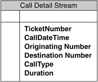
The business needs to analyze the data across all dimensions. The data is provided in a call detail record (CDR). The solution will eventually need to handle billions of rows in the fact table and be able to load and transform millions of facts per day. Recent data is queried far more often and at more detailed levels than historical data. However, queries summarizing current data and comparing it with parallel historical periods are also common, and need to perform well.
Data is kept for five years before being archived.
Data is generated nonstop, 24 hours per day. Analysts in three time zones expect access between 6 a.m. and midnight. At best, three hours are available during which the solution can be offline. However, taking the database offline would create a serious backlog of data waiting to be loaded, so this is not a viable option. Backups and other maintenance procedures still need to be performed, but with minimal impact on performance.
The operations staff who works with the data warehouse need the capability to easily remove and archive older data as it becomes less relevant, without requiring extensive reprocessing. Also, backups in general consume a lot of disk space before being transferred to offline storage. This space needs to be cut in half.
Our customer’s database is essentially overwhelmed by the data volume, forcing a reduction in detail just to be able to keep up. Much of the problem can be attributed to the time required to back up the data and reorganize the indexes. You might be asking yourself why we need to back up and perform index maintenance on all the data. After all, haven’t we already done that for all but the most recent data? The historical data hasn’t changed; we are just adding new data. If we could find a way to do the maintenance only on the new data, we could reduce the time for maintenance to almost zero. Figure 11-1 shows the components that are influential in supporting a VLDB.
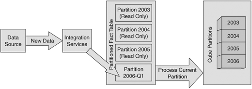
The core of the architecture supporting very large databases is partitioning of the relational tables and OLAP cubes. Each partition can be treated somewhat independently. This provides the opportunity to design shorter maintenance operations, faster backups, higher performance-loading OLAP cubes, and potentially more efficient querying.
In SQL Server, a partitioned table appears as a single table to a user, but the rows in the table are physically divided across a number of separate partitions. Partitioning the table can offer better performance through parallel operations. Partitions make it easier for you to manage the table because you can work with subsets of the data rather than the entire table.
Using multiple partitions associated with multiple filegroups in the data warehouse, we can dramatically improve backup times and maintenance times. A filegroup is simply a collection of files that you can use to distribute data across your available storage. Using filegroups, we also save a substantial amount of disk space that would be consumed by a full database backup. This comes from our capability to mark partitions read-only, which we will never have to back up or reorganize the indexes more than once. We only have to back up and maintain a relatively small “current” partition.
The cubes in the Analysis Services database will be partitioned in a manner similar to that of the relational database. This will allow us to import just the new data into a “current” partition, and process only the data in that partition. All the historical data will not need to be processed. The data in the cube will be online continuously, and only a small amount of resources will be consumed in the reprocessing.
In our ETL processing, we will use the native high-speed pipeline architecture of Integration Services where it is advantageous, but trade some of the clarity and maintainability of using Integration Services transformations to take advantage of the performance of set operations performed by SQL queries.
One thing we need to do to guarantee good load performance is to make sure only the changes to the data are loaded, whether it is new facts or dimensions. At least, we should only have to reload a very small portion of existing data. We impose a business rule that no fact data is ever updated, because that would mean reprocessing all the data in the same partition. If a change is needed, a new fact containing the positive or negative adjustment required is used, as described at the end of Chapter 8, “Managing Changing Data.” If dimensions change, consider whether they are Type 2 changing dimensions, where you create a new instance of the member rather than change an existing member’s attributes.
With the capability to manage larger volumes of data, we can now support the storage of more detailed data. However, this leads us into our next problem: longer query times.
As you have seen in previous chapters, Analysis Services is designed to precalculate aggregations of values to one or more levels, such as summing up the call duration to the month or quarter level. This means that a query no longer has to touch each row to determine the duration of all the calls per quarter. By using Analysis Services and taking advantage of the aggregations, we can meet the performance criteria for most queries. Analysts will be able to use Excel, Reporting Services, or other third-party tools to query the Analysis Services databases.
Before you add or change resources to improve performance, it is important that you determine what constraints your application is experiencing. Usually, the bandwidth of the path to and from your mass storage, memory for caching data, and processor cycles is the resource constraint. The bottleneck tends to occur during the access to mass storage, because it is the slowest of all the resources. However, it is important that you monitor your system to determine which resources are hitting its limit. You can use Windows System Monitor to view the utilization of resources. In addition, you want to make sure that your application is using efficient queries and techniques. You can use SQL Profiler to look for long-running queries.
To improve immediate performance, increase the memory of the data cache. This is often the best choice. In a 32-bit system, your available memory is constrained by the architecture. This is not the case with 64-bit architecture. In the near future, 64-bit processors will be the norm, and you won’t need to decide whether you need one, or you can get by with a 32-bit processor. Currently, price and some application restrictions mean you still need to evaluate this option. In our example, we were not constrained by memory. Yes, there is a large volume of data, but much of it is historical and not referenced often. Our dimensions are relatively small, and our partitioning scheme means we do not have to reprocess much data. We therefore can continue to use a 32-bit architecture.
The solution will deliver the following benefits to the client:
-
Increased efficiency and profitability through the capability to identify network route utilization trends and deploy equipment for optimal capacity
-
Identify marketing opportunities where excess capacity could be promoted and premiums charged for prime routes and times
We focus on the fact table in discussing the data model. The fact table is usually the largest table and therefore the most obvious candidate for partitioning. The dimension tables in our case are small and will not benefit from partitioning.
Our logical schema doesn’t change significantly from what you might expect, but the physical implementation is very different. Partitioning requires a column that we can use to direct rows to a specific partition, so you do need to be sure you have an appropriate column. We are going to partition by date, and the CallDate column fulfills that requirement.
We have paid some attention to ensuring the data types are as small as possible to keep the row size down. This is not so much for saving disk space as it is for performance. The more rows you can fit on a page, the better the performance. Even if you have a relatively “small” VLDB with just a billion rows, each byte you save is a gigabyte you don’t have to store or back up.
Our fact data sources are flat files, each containing call detail data from one of a number of on-line transaction processing (OLTP) servers, as shown in Figure 11-2.
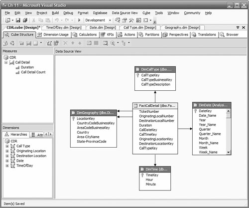
In the fact table shown in Figure 11-3, we have converted the phone number into two parts: the area code, which we will use to determine the general location of the call; and the local number. This allows us to have a Geography dimension with a key that is independent of the phone number business key. Area codes are well defined and can be imported from standard industry sources. We have split date and time apart because we want independent date and time dimensions. We chose to use a data type of smalldatetime for the call date to shorten the row length. The range of dates is from 1900 to 2079, which suffices for our purposes. The Time dimension key can be computed as the number of minutes past midnight, saving a lookup.

Our fact table has no declared primary key or unique key. This isn’t unusual in a fact table, but in this case we can’t have one. This is because of a restriction imposed by partitioning. Any columns in unique indexes must be part of the partitioning key. If we were to create a unique surrogate key to be used as a primary key, we would have to include it in the partitioning criteria. We don’t want to partition by an arbitrary number, so even if you are in the habit of putting primary keys on your fact table, you will probably want to skip it this time. You can, and should, create a nonunique clustered index on the date column. If you must have a primary key, you can work around this restriction. Create a compound primary key using the date (or whatever column you are partitioning by) and any other unique column. If you don’t have a unique column, create a surrogate key using a column with the Identity property set to true.
We’ve always recommended that you don’t have a surrogate key for the Date dimension. This scenario is a good example of why, because we want to have a clear understanding what data is in our fact table partitions. The partition contents are defined by a key range, and Date is a human-readable value. A surrogate key wouldn’t necessarily tell us directly what dates are in the partition. We also want the partitioning function to be easily read and maintained, and dates are more understandable than the IDs we would generate for a surrogate key.
Our Analysis Services database follows our data warehouse schema closely, as shown in Figure 11-4.
Now we look in detail at our proposed solution. We start with how to design, create, and manage the partitioned tables in the data warehouse. Next, we look at the ETL processes we need to create to populate the tables in the data warehouse. Finally, we look at how to design, create, and manage the partitions that make up the cubes.
You use partitioned tables for optimizing queries and management of a large relational table. Our partitions will be based on date because our usage of the data is primarily for a specific data range.
To design partitions, you need to decide on a basis for the partitioning. What you are looking for is one or more attributes in the table that will group your data in a way that maximizes the specific benefits you are looking for. In our example, we are looking for the following:
-
Fast load time
-
Minimal impact on availability when loading data
-
Acceptable response time as database size increases
-
Minimal impact performing any maintenance procedures such as index reorganization
-
Minimize backup time
-
Easily archive old data
A partitioning scheme is frequently based on time because it can support all of the benefits listed above. Each partition would hold data from a specific time period. If the data in a partition does not change, you can mark the file group read-only, back it up once and not have it take time and space in future backup operations. If you need to purge or archive old data, you can easily remove the partition without having to perform a costly delete operation.
Your partition sizes normally are determined by the amount of data estimated to be in a partition and a convenient time period. Larger partitions make management a bit easier, but may contain too much data to provide us with the efficiency we are seeking. Daily or weekly partitions are common. In this example, we will create uniform weekly partitions. It can take up to four weeks to receive all the data, so we will keep the prior four partitions writeable, and mark old partitions read only. This will mean we only need to back up four weeks of data.
No GUI exists for creating the partition function or the partition scheme, but even if there were, we still recommend that you use scripts to create partitioned tables so that you have a repeatable process. Here is an overview of the steps you take:
-
Create a partition function.
-
Create the filegroups.
-
Add files to the new filegroups.
-
Create the partition scheme.
-
Create the partitioned table.
The partition function defines the boundary values that divide the table between partitions. You specify a data type that will be passed to the function, and then a number of values (up to 999), which are the boundary points. The name of the partition function is used later when you create the partition scheme. To illustrate the idea, the example below creates six partitions on a weekly basis, with the last partition holding everything beyond January 29.
CREATE PARTITION FUNCTION PartitionByWeek (smalldatetime)
AS RANGE RIGHT
FOR VALUES (
'2005-DEC-25',
'2006-JAN-01',
'2006-JAN-08',
'2006-JAN-15',
'2006-JAN-22',
'2006-JAN-29')
The partition function that you create determines which partition a row belongs in. Partitions don’t have to be uniform in size. You can have partitions for the current four weeks, previous month, and another for everything else in a history partition if that suits your query profile. You can also specify more filegroups than you have partitions. The extra ones will be used as you add partitions.
A filegroup is simply a set of one or more files where data or indexes can be placed. A filegroup can support more than one partition, and a partition can be distributed over more than one filegroup. In our example, we use one filegroup for each partition. The partitions were defined by the partition function we just created previously. We will create one partition for each of the ranges defined in the function. We will add one file to each filegroup:
—Create "FG2005WK52" Group
ALTER DATABASE CDR
ADD FILEGROUP FG2005WK52;
GO
—Add file "CD2005WK52" to FG2005WK52 group
ALTER DATABASE CDR
ADD FILE
(
NAME = Archive,
FILENAME = 'D:CDRDataCD2005WK52.ndf',
SIZE = 3000MB,
FILEGROWTH = 30MB
) TO FILEGROUP FG2005WK52
GO
ALTER DATABASE CDR
ADD FILEGROUP FG2006WK01;
GO
ALTER DATABASE CDR
ADD FILE
(
NAME = CD2006WK01,
FILENAME = 'D:CDRDataCD2006WK01.ndf',
SIZE = 3000MB,
<a id="page_355/">FILEGROWTH = 30MB
) TO FILEGROUP FG2006WK01
GO
.
.(repeat for the remaining partitions)
We expect that 3,000MBs is sufficient space for one week’s data. If that’s not enough, the file will grow by 30MB whenever it runs out. In SQL Server 2005, the new space is not formatted when it is allocated, so this operation is quick. Having multiple files in each filegroup would allow for some parallelism in query execution. If you have enough drives, you could spread the load across multiple drives. With high data volumes, such as we anticipate here, you will likely be using SAN storage with many drives and a large cache.
Now, you need to map the partitions to filegroups. You can map them all to one filegroup or one partition to one filegroup. We will assign each partition to its own filegroup because that will give us the performance and manageability we are seeking. The partitions and filegroups are associated one by one, in the order specified in the filegroup list and in the partition scheme. You can specify more filegroups than you have partitions to prepare for future partitions:
CREATE PARTITION SCHEME WeeklyPartitionScheme
AS PARTITION PartitionByWeek
TO (FG2005WK52, FG2006WK01, FG2006WK02, FG2006WK03,
FG2006WK04, FG2006WK05, FG2006WK06)
With the partition scheme now created, you can finally create a partitioned table. This is straightforward and no different from creating any other table, other than to direct SQL Server to create the table on a partition schema:
CREATE TABLE [Call Detail]
(TicketNumber BigInt NOT NULL,
CallDate SmallDateTime NOT NULL,
...
)
ON WeeklyPartitionScheme (CallDate)
In Figure 11-5, you can see how all the pieces fit together to store the data in a table. When a row arrives for insert, the database engine takes care of figuring out where it should go without any further work on your part. The partition column is used by the partition function to determine a partition number. The partition number is mapped by position to one of the partitions in the partition schema. The row is then placed in a file in one of the filegroups assigned to the selected partition. To reduce clutter in the diagram, we haven’t shown all the files or filegroups.

You can also partition indexes. By default, indexes are partitioned to be aligned with the data partitions you created. This is the most optimal configuration. If your data and index partitions are not aligned, you cannot take advantage of the efficiencies offered by filegroup backups.
You need to be aware of some restrictions when designing the data model for your application. We have outlined the important ones here.
Tables that are currently separate that you are planning to merge into a partitioned table should be essentially identical, with few exceptions. For example, if you have two tables, current and historical, and you plan to merge current data into a partition in the historical data table, you can’t add additional columns to one table to support some functionality for current data and not carry the columns over into the historical data table.
There can’t be any foreign key constraints between tables you are planning to combine into the same partition. This restricts you from having self-referencing relationships in the model.
There can’t be any foreign key constraints from other tables to a table that could be merged into another partition. An example of this would be a dimension table that is referenced in a constraint by a fact table. You are unlikely to have this situation in the portion of a data warehouse that is supporting a dimensional model. The fact table is usually the table you would be partitioning, and the foreign key relationships are usually from the fact table into a dimension table. Dimension tables generally are small enough that you do not need to partition them.
Indexed views are not allowed in either the source or the target, because schema binding is not allowed. If indexed views were implemented to improve the performance of an application, a cube built based on the data warehouse should be able to provide the same if not better performance gain.
The pipeline architecture of an SSIS data flow is extremely efficient in loading and transforming data. After we have covered how the package is put together, we look at ways we can optimize it for high-volume data flows.
When talking about large volumes of data, bulk load or bcp utilities always come to mind. You can also use a Bulk Load task in your control flow. However, we want to transform the data, so these approaches won’t help us.
Let’s look at an SSIS package that can be used to import data from a text file and insert it into a data warehouse using the Fast Load option. This isn’t strictly a VLDB solution, but it’s an opportunity to show you another way of loading data. Flat files are a common way of recording or delivering larges volumes of data.
The first thing you need to do is to create a connection manager that points to your CDR input files. In the Connection Manager panel at the bottom of the window, right-click and then choose New Flat File Connection. Give the connection manager a name such as CDR Input. Browse to a file containing CDR data and select the file. Set the format to match your file. In our example, the columns have fixed width, and we just need to define the width of each column. If your data has a separator between columns, such as a tab or comma, choose delimited for the format. On the Columns tab, drag the red line to the right until you reach the end of the row. To define a column break, click the ruler.
Try to get the column breaks set correctly before assigning names to the columns. After that point, you need to use the Advanced tab to create new columns and set their widths, as shown in Figure 11-6.
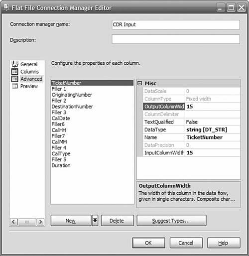
When you are configuring the Advanced column properties, take care to select the right data type. The default is DT_WSTR, which is a Unicode or nvarchar data type. Clicking Suggest Types helps if you have many columns that are not character types. The name of the column is also set on the advanced properties. If you don’t set the name, you will have a list of columns named Column 0 to Column n, which won’t make it easy to maintain your package, so we strongly encourage you to supply names here.
Now you need to create the Data Flow task to extract the data from the CDR flat file, apply some transforms to create the keys in the fact table to link to the dimensions, and then insert the rows into the fact table in SQL Server.
We want to transform the originating and terminating country and area code into surrogate keys that reference our Geography dimension, and also transform the Call Type to a surrogate key that references our Time dimension, Date dimension, and Call Type dimension. We use a Lookup data flow transformation to do this.
We start the data flow by defining the flat file source to reference the “CDR Flat” connection we defined previously. We connect its data flow to the first lookup task. Each Lookup task does one transform. The updated rows are passed on to the next Lookup task, until all transforms have been completed. The last Lookup transform is connected to a SQL Server destination connection, which writes the rows to the data warehouse. Figure 11-7 shows the data flow.
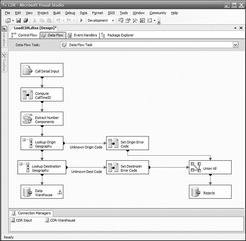
On a Lookup task, SSIS tries to read as many rows as possible and perform in-memory operations. In the data flow shown above, each batch is processed by the first Lookup task and then passed on to the next Lookup task. The first Lookup task loads another batch, and the pipeline begins to fill as each Lookup task passes its results to the next task.
The Lookup data flow transform will try to use as much memory as is available, to enhance performance. You can restrict the amount of memory used for cache, but full caching (the default) is normally recommended if you have the memory.
If the reference table is very large, you may run out of memory and the lookup transform will fail. You can reduce the memory required by using a query instead of a table name for the reference table. In the query, select only the columns you are mapping to and the ones you want to look up. If that doesn’t help, you can set the caching mode to Partial. Partial caching loads the rows from the reference table on demand (that is, when they are first referenced). In the Lookup transform that determines the PlanType, we have to reference the Customer table by the Origin Area Code and the Origin Local Number. Because the fact data is loaded so frequently, only a small number of customers show up in the CDR data, but those who do often make many calls. This is the kind of situation where partial caching may prove to be very useful. You set the caching mode either through the Advanced Editor or in the Properties window of the Lookup transform.
To optimize the data flow, don’t select columns that you do not need, either in the data source or in lookups. In a union all transform, you can drop columns that you no longer need.
As discussed in Chapter 4, “Building a Data Integration Process,” SSIS Lookup transformations provide many advantages over loading the new fact data into a staging area and then joining to the dimension table using SQL to fetch the surrogate keys. Lookups are easier to understand and maintain, and they enable you to handle errors when the reference table does not have a matching row. Joins are generally faster than lookups, but for smaller data volumes, we were willing to sacrifice some performance for the clarity and error handling, because the total difference in time was relatively small. For extremely large reference tables, a join may be so much more efficient that the time difference is substantial, and you have no choice but to implement a translation using a join. You should do some testing before committing to either solution. In the case of a join, implement the join as an outer join so that you don’t lose any facts.
You could implement a join either by creating a view in the source database or in the SSIS data source. Often, you don’t have the permission to create a view in the source database, so you must create the appropriate SQL statement in the SSIS data source. You create your own SQL statement by selecting SQL Command, instead of Table or View, in the connection manager. You can type in the SQL directly, or you can use a graphical wizard to help you create the query. But there are some issues with doing joins in the query in the OLE DB data source. You usually join incoming facts to the dimension tables in the data warehouse. You have to explicitly name the source database in the query, and this makes it difficult to migrate to other environments without changing your package.
In our case, we can’t use a join because our data source is a flat file. We have the option of using the Bulk Insert task to load the flat file into a temporary table and then performing the joins to the dimensions using that table. You don’t need to spend time to index the temporary table because every row will be read, so the indexes won’t be used.
If you are using an OLE DB destination, choose the Data Access Mode Table with Fast Load option. This option offers a significant performance enhancement over the standard Table or View option. If you are running the package on the same server as SQL Server, you can choose a SQL Server destination, which will provide further performance improvements.
Cube partitions enhance performance and manageability. They are invisible to users of the cube, so you have complete freedom to design and manipulate partitions according to your needs. Partitions offer the following advantages when working with cubes:
-
Parallel loading of partitions.
-
Only partitions that have been updated need to be processed.
-
Easy to remove old data by simply deleting a partition.
-
Different storage models can be applied to each partition. You could use a highly efficient multidimensional OLAP (MOLAP) for historical partitions, and relational OLAP (ROLAP) for real-time current partitions if necessary.
-
Queries can be more efficient if only a few partitions are needed to satisfy them.
In our example, we want to be able to efficiently add new data, while minimizing the impact on cube users. Smaller partitions perform better than larger ones, although it may mean a bit of extra management overhead. Ten to 20 million facts per cube partition is a good rule to follow. If you have queries that limit a search to one or a few partitions, it will be faster than if the query has to search one large or many small partitions. To improve performance, your objective is to create small partitions that cover the span of the most frequent queries. To improve maintainability, you want as few partitions as possible.
Weekly partitions are a good compromise between manageability and efficiency, so we’ll implement uniform weekly partitions just as we did for the relational table.
You can create cube partitions using the BI Development Studio or SQL Server Management Studio. You can also use the Integration Services Analysis Services Execute DDL task to execute commands to manage cube partitions. We’ll use BI Development Studio while we’re developing our solution so that the partition design is captured as part of our source code. You will first have to modify the default partition’s source so that it doesn’t reference the entire call detail table. Next, you create additional partitions as necessary according to your design.
Because you have multiple partitions, you need to have an independent table or view for each partition, or a query that is bound to the partition. The data returned by the tables, views, or queries must not overlap; otherwise, the cube will double-count those rows.
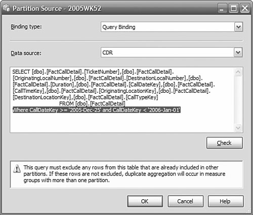
For all our partition sources, we are going to use Query Binding rather than Table Binding. Query Binding enables us to use a single fact table as the data source, and then a where clause to restrict the call detail rows to a date-range matching the partition. You would use Table Binding if each partition had its own separate relational table as a data source.
To make sure there is no data overlap in the queries for each partition, we use a where clause like this:
CallDate >= '1-Jan-2006' and CallDate < '8-Jan-2006'
The use of >= to start ensures we capture every call that begins after midnight on January 1. The use of < for the end date ensures we capture all the calls right up to, but not including, January 8. If we had used <= '7-JAN-2006', we might miss calls made on January 7 if the time component in the fact table wasn’t 00:00. We don’t expect the time to be anything else, but this is defensive design in case future developers modify (or ignore) the design assumptions. We also won’t use clauses like
CallDate BETWEEN '1-Jan-2006' and '8-Jan-2006'
CallDate BETWEEN '8-Jan-2005' and '15-Jan-2006'
because the ranges overlap at the endpoints and the facts on January 8 would be duplicated in adjacent partitions (in this example, 8-Jan-2006 would be included by both of these where clauses).
TIP:
Avoiding Gaps in Partition Ranges
A good practice to follow is to use the same value in the predicate for the boundary, but omit the equality comparison in one of the predicates. For the earlier partition, use less than (<), and for the later partition, use greater or equal (>=). An earlier partition includes facts up to but not including the boundary value. The later partition includes facts at the boundary value and greater. That way, there is absolutely no gap and absolutely no overlap. If there are gaps, you will have missing data, and if you have overlaps, you will have duplicate data.
QUICK START: Creating the Analysis Services Partitions
Start BI Development Studio and open your Analysis Services solution. Now, we’ll go through the steps to create the partitions for your cube:
-
Choose the Partitions tab. Click the Source field of the initial partition, and then click the ellipses. Select Query Binding in the Binding type drop-down. Add the appropriate predicate to the where clause, as shown in Figure 11-8.
-
Add the additional partitions. Click New Partition to start the Partition Wizard. Choose the measure group that will reside in the partition. There is only one in our example. Next choose the Partition Source—the table that will supply the data for the partition. If you have many tables, you can specify a filter to reduce the length of the list you have to choose from. Check the table in Available Tables, and then click Next.
-
Be sure the check box is selected to specify a query to restrict rows. Supply the predicate for the where clause to limit the rows you will allow into this partition, as you did in Step 1. Click Next.
-
Accept the defaults for the processing and storage locations. Click Next.
-
Provide a meaningful name for the partition that will help you identify its contents. Select “Copy the aggregation design from an existing partition.” If you are creating the first partition of its kind, choose Design aggregations now. Leave “Deploy and process now” unchecked. Click Finish.
-
Continue adding the partitions you need, repeating from Step 2.
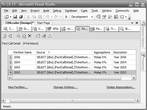
You should end up with a set of partitions similar to Figure 11-9.
You must now deploy the solution for your changes to be visible to other applications.
Aggregations are used by Analysis Services to improve response time to queries that refer to a rollup of one or more measures. For example, Sales by month or quarter is logically rolled up by summing Sales by day. If Analysis Services precalculates the Sales by month, then to get Sales by quarter, only three values (for the three months in a quarter) need to be summed. If some aggregations are good, are more aggregations better for large cubes? Not necessarily!
The number of potential aggregations in your cube depends on the number of dimensions, attributes, and members in your dimensional model. It is not possible to precalculate all aggregations for most cubes because the number becomes astronomical quickly. The more aggregations that are stored, the better your performance, but it will also take longer to process new data, and partition size will increase.
Remember that you must specify the attribute relationships in your hierarchies for good aggregations to be created. This is particularly important in large databases. Refer back to Chapter 5, “Building an Analysis Services Database,” to review how to set up the relationships.
Partitions can each have their own aggregation designs. This enables you to tailor the aggregations differently if you find, for example, that users pose different queries against historical data than for current data. However, a caveat applies here. When you merge partitions, they must have the same aggregation design. That is why we copied aggregation designs from other partitions when we created them.
In BI Development Studio, you can find the tool for designing aggregations on the Partitions tab of your cube. When you first design aggregations, Analysis Services creates a set of aggregations that it estimates will improve performance. You can specify how much space you are willing to provide for aggregations or how much performance improvement you want. You must limit the aggregations if the processing time becomes unacceptable. Consider starting with something like a 20 percent improvement.
Regardless of the initial aggregations you set up, when in production, you want to be sure the aggregations are appropriate for the queries that your users are sending. Analysis Services provides a means to do this, called Usage Based Optimization, or UBO. We describe how to use UBO in the section on “Managing the Solution” at the end of this chapter.
SQL Server 2005 Analysis Services has a much higher limit on the number of members that can belong to a node in a dimension compared with Analysis Services 2000. However, if you have a GUI interface that allows a user to drill into dimension levels, this might create a problem for the interface or the user, or both. You should consider very carefully whether you want to design such a large, flat dimension. If you can find a natural hierarchy for a dimension, it is usually better to implement it.
In our example, LocalNumber could be very large—seven digits means potentially ten million members. However, we don’t need to use LocalNumber to solve our business problem, so we won’t include it in a dimension. If it had been necessary, we could create a hierarchy that included the three-digit exchange number as one level and the four-digit subscriber number as a child of the exchange.
In a well-designed partitioned solution, it is easy to manage partitions. In a poorly designed solution, you can face huge performance issues moving large amounts of data between partitions. The most important consideration in designing your solution is to plan and test it end to end on a small amount of data.
You will see some performance benefit during the initial loading of large tables, if you create the table indexes after the initial loading is complete. When you create the indexes, be sure to create the clustered index first; otherwise, you will pay twice for the creation of the nonclustered index. You need to have about 150% more space for a work area when you create a clustered index on a populated table.
You need to create the table partitions for the weeks that are in the initial load.
On a regular basis and as quickly as possible, you will want to mark filegroups to read-only so that they won’t require any more maintenance. You also need to create the partitions for the upcoming periods.
In the following section, we discuss some of the other activities necessary for keeping your system working well, such as the maintenance of the indexes of the active partitions, how to move old data out of the table, and an optimal backup strategy that avoids repetitively backing up unchanged historical data.
If data in a partition is changing frequently, the indexes can become fragmented and index pages will not be full, which reduces performance. After you have populated a partition with all the data for its prescribed time period, consider performing an index reorganization to remove the empty space on index and data pages. One of the advantages of partitioning a table is that you can perform index maintenance on a single partition. If most of your partitions are historical, and so they haven’t changed, they will not need to have any index maintenance performed on them. You only need to consider the current partition for maintenance.
You can tell how fragmented an index is using the system function sys.dm_db_index_physical_stats. For example, to see the fragmentation in the indexes in the Call Detail table, execute this statement:
SELECT IndexName, AvgFragmentation
FROM sys.dm_db_index_physical_stats (N'dbo.[Call Detail]',
DEFAULT, DEFAULT, N'Detailed'),
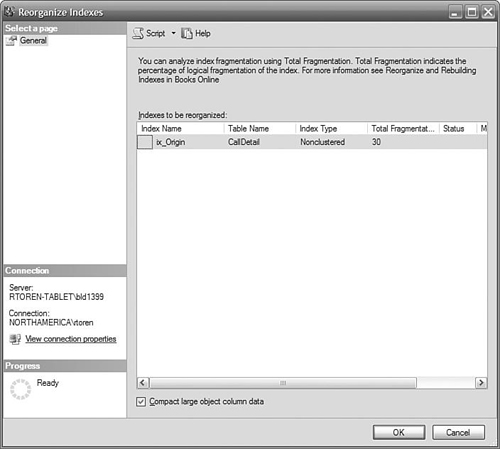
You can view index fragmentation or rebuild or reorganize an index in SQL Management Studio by right-clicking the index in the Object Explorer and choosing Rebuild or Reorganize, as shown in Figure 11-10. As a rule of thumb, you would choose to reorganize an index if the fragmentation were less than 30 percent, and you would rebuild it if the fragmentation were greater than 30 percent. You can target all indexes by right-clicking the Index node rather than a single index.
When a partition contains all the data for its time period, you can mark the filegroup where it resides as read-only. After you’ve performed a final backup of the partition’s filegroup, you will never have to back up this data again.
You set the read-only flag on a filegroup using the Management Studio. Right-click the database and choose Properties. Next, select the Filegroups page and check the Read-only box. Then choose OK.
Users cannot be connected to the database when setting the Read-only flag on a filegroup, so you will have to perform this operation during a scheduled maintenance period.
When it is time to remove old data, you can delete the data one partition at a time. This is a highly efficient way of removing data, but it is a nonlogged operation, so you can’t undo it.
You remove data in a partition by using the ALTER TABLE ... SWITCH PARTITION command to move the partitioned to a nonpartitioned table and then deleting the table. For example, to change the data in the partition containing the data for the date Dec 31, 2004 to a non-partitioned table that you can subsequently drop, execute this command:
ALTER TABLE FactCDR $Partion.PartitionByWeek('31-Dec-2004')
SWITCH PARTITION TO EmptyTable
EmptyTable must already exist, have the same schema as the FactCDR table, and be empty. This command will execute very quickly, as will the Drop Table command.
Backup works with databases or filegroups, not partitions. Because we designed our partitions to each occupy their own filegroup, you can back up each filegroup independently. In addition, we have marked historical partitions to be read-only, so we don’t have to back them up more than once. Our backup and restore times are now shorter.
In our example, source data arrives in frequent batches throughout the day. Because we have the source data available, we have the option of rebuilding the data from the last full backup and reloading the source data files. This would allow us to use the simple recovery model. In our example, we encourage using a bulk-logged recovery model, for manageability and faster recovery times. It is much easier to determine which log files need to be applied to restore the database than to determine which data files need to be reloaded. It is also faster to restore the database from log files than to reload the data.
If you do infrequent bulk loading of data into your data warehouse, you may be able to set the database recovery model to Simple. By infrequent, we mean a few times per day, but more than once or twice per day. This can reduce the amount of space consumed by the log file over a daily load. The more frequently you load data, the smaller the log file, but you will have to do more full backups, too. If you have not partitioned your warehouse so that the partition for “current” data is small, there may be little or no advantage in doing backups after loading data. To take advantage of the Simple recovery model, you must perform a backup of the modified partition immediately after you perform a load. If you do any loading by trickling in data, you should not use the Simple recover model; instead, choose Full, and then you will also need to perform log backups on a regular basis.
Table 11-1 presents our backup plan, which minimizes the amount of data you need to back up and provides for a faster recovery in the event you have to restore the data. Note that you do not have to back up the historical partitions.

Partitions are continuously changing in an Analysis Services solution. You receive new data, want to archive old data, move current data to historical partitions, or perhaps your users have changed their query patterns and you need to reoptimize for those new queries. In this section, we discuss the ongoing management of partitions.
Remember that any changes to partitions that are made using SQL Server Management Studio are not reflected back into your Visual Studio projects. You will have to create an “Import Analysis Services 9.0 Database” project to create a project that matches the current design. If you deploy the original project, you will overwrite any changes you have made to the cube.
When you process a partition, it reads the data specified by the source you defined when you created the partition. You can start processing a partition manually, under program control, or by a task in an SSIS package. You only need to populate partitions where the data has changed.
The ETL processes load data into one of the four recent weekly partitions. We fully process these partitions to bring in the new transactions. We can get away with this because it is only four week’s transactions, not the entire five years. The prior periods in the relational table are read-only and therefore don’t need processing.
A property you will want to set to improve processing times is the RelationshipType. This is a property of an attribute relationship in a dimension. For example, this is a property of the Quarter relationship to Month in the Date dimension. This property has two values: Flexible and Rigid. Rigid relationships offer better query performance, whereas Flexible relationships offer better processing performance in a changing dimension. If a member will not likely move in the hierarchy, as would be the case with dates, you can set the RelationshipType to Rigid. If a member does move in a rigid relationship, an error is raised. The default is Flexible.
You can initiate dimension processing manually by right-clicking the dimension in the Solution Explorer and choosing Process. You can also use an SSIS task or an XML/A command to process a dimension.
You can merge smaller partitions into a larger historical partition to reduce your administrative overhead, although at some point you will see a degradation in performance.
To merge a partition into another partition, the partitions need to have similar aggregation designs. The way we created our partitions, aggregation design is inherited from the previous partition, so your designs should match up properly. If you want to change the aggregation design of a partition, wait until it is “full”—that is, you aren’t going to add any more partitions. Then you can redesign the aggregations because it’s not going to be merged with any other partition. If you want to copy the aggregation design from another partition, you can do that in Management Studio. Drill down into the cube, through the measure group, down to the partition you want to change. One of the right-click options is to copy the aggregations.
The business requirements state that at least five years of data should be kept. At the end of each year, you can remove the oldest year partition, which now contains the fourth year of data.
You can delete a partition using Management Studio by right-clicking the partition and then choosing Delete.
None of the aggregations built initially are based on anything but an educated guess by Analysis Services based on factors such as the number of members in the dimension. What you really want is an aggregation design based on actual usage. Fortunately, Analysis Services can track the queries being submitted by your users. You can use the Usage Based Optimization (UBO) Wizard to read the query log and design a better set of aggregations based on actual usage. UBO is done on a per-partition basis.
Before you can do UBO, you need to start collecting data in the query log. You enable this in the properties of the Analysis Services server. Look for the property Log Querylog CreateQueryLogTable and set it to true. Next, set the value of Log Querylog QueryLogConnectionString to point to a SQL Server table where you want to record the queries to be used for profiling. You want to collect data for a long enough period to provide a good cross-section of queries, but it’s not recommended that you run with logging enabled all the time.
After you’ve collected data, you can have the UBO Wizard analyze the log and recommend some aggregations. You start the UBO Wizard from SQL Server Management Studio. You need to drill down from the cube, through the measure groups, to locate the partitions you want to optimize. Right-click a partition, or the Partitions node, and choose Usage Based Optimization. In the wizard, you can filter the data in the query log by date, user, or set of most frequent queries.
Here we provide some additional avenues for you to consider to improve your solution, after you have implemented the basic elements of this chapter.
In this chapter, we described a scenario where the data is constantly arriving, or at least arriving very frequently in batches. Our purpose was to describe the ways you can efficiently process high volumes of newly arriving data and be able to query large databases efficiently. We want to leave you with some ideas on how to detect when new data has arrived. In Chapter 4, we discussed how you can browse a directory for files and pass a filename into a Data Flow task. Here are some other avenues you can explore:
-
Two Control Flow tasks that you can look at for detecting file arrival are the Message Queue task and the WMI Event task.
-
Chapter 12, “Real-Time Business Intelligence,” on real-time OLAP describes methods for automatic background processing of cube partitions when new data arrives.
-
A complete object model exists for working all aspects of partitions, ETL packages, and cubes. You can quickly build an application to automate the processing of data from the arrival of the flat files through to incrementally processing the cubes and creating new partitions in any language supporting the Common Language Runtime (CLR).
As noted in the introduction, you can also use partitioned views (PVs) to partition your data. This allows you to create a unified view of a table distributed over multiple databases. You can now manage each partition of the data independently. If the databases are on other servers, you have a distributed partitioned view (DPV). The advantage of DPVs is that the load can be distributed over several servers, and the partitions are searched in parallel. Each table has a constraint similar to one boundary point in the partition function. The individual tables are combined in a view that unions the tables together. This makes the use of the partitioned view transparent to a user. Select statements issue parallel queries to the relevant partitions. Data inserted through the view will be inserted into the table on the correct server.
The databases do not need to contain all tables, only the tables you want to divide into partitions. By using all but one database for historical data, you can find some operational benefits. If your partitioning is by time, you can reduce the backup time by marking the historical databases read-only; then, you only need to back up a much smaller current database.
You should consider PVs and DPVs only when you have extremely large databases, and queries that usually require data from only a few partitions. PVs, which by definition do not involve the network, are less resource intensive than DPVs. DPVs allow you to scale out over several servers, but the cost of initiating a query to another server across the network is relatively high compared to a PV or local query, so you should measure the performance of a DPV to ensure you are receiving a benefit from this design.
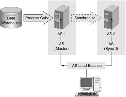
You can deploy the same database on several Analysis Services servers using Database Synchronization. This increases the number of users that you can handle. In this scenario, the Analysis Services servers have identical but separate databases. The partitions exist on locally managed storage (which could be a storage area network [SAN] drive). Each server has its own IP address and service name, but also has a virtual IP and virtual service name provided by the load-balancing service. The load-balancing service is either Windows NLB or a hardware device such as an F5 switch. Figure 11-11 shows a typical configuration.
You can initiate synchronization from SQL Server Management Studio by right-clicking the Databases node of the target server (not the source server). You then specify a source Analysis Services server and database you want to synchronize with. Using the same wizard, you can create a script to enable you to schedule periodic synchronizations.
During synchronization, both the source and the target can continue to be queried by users. When synchronization finishes, Analysis Services switches users to the new data, and drops the old data from the destination database.