
Audio Electronics
Audio electronics, in part, deals with converting sound signals into electrical signals. This conversion process typically is accomplished by means of a microphone. Once the sound is converted, what is done with the corresponding electrical signal is up to you. For example, you can amplify the signal, filter out certain frequencies from the signal, combine (mix) the signal with other signals, transform the signal into a digitally encoded signal that can be stored in memory, modulate the signal for the purpose of radiowave transmission, use the signal to trigger a switch (e.g., transistor or relay), etc.
Another aspect of audio electronics deals with generating sound signals from electrical signals. To convert electrical signals into sound signals, you can use a speaker. (If you are not interested in retaining frequency response—say, you are only interested in making a warning alarm—you can use an audible sound device such as a dc buzzer or compression washer.) The electrical signals used to drive a speaker may be sound-generated in origin or may be artificially generated by special oscillator circuits.
15.1 A Little Lecture on Sound
Before you start dealing with audio-related circuits, it is worthwhile reviewing some of the basic concepts of sound. Sound consists of three basic elements: frequency, intensity (loudness), and timbre (overtones).
The frequency of a sound corresponds to the vibrating frequency of the object that produced the sound. In terms of human physiology, the human ear can perceive frequencies from around 20 to 20,000 Hz; however, the ear is most sensitive to frequencies between 1000 and 2000 Hz.
The intensity of a sound corresponds to the amount of sound energy transported across a unit area per second (or W/m2) and depends on the amplitude of oscillation of the vibrating object. As you move further away from the vibrating object, the intensity drops in proportion to one over the distance squared. The human ear can perceive an incredible range of intensities, from 10-12 to 1 W/m2. Because this range is so extensive, it is usually more convenient to use a logarithmic scale to describe intensity. For this purpose, decibels are used. When using decibels, sound intensity is defined as dB = 10 log10 (I/I0), where I is the measured intensity in watts per meter, and I0 = 10−12 W/m2 is defined as the smallest intensity that is perceived as sound by humans. In terms of decibels, the audio intensity range for humans is between 0 and 120 dB. Figure 15.1 shows a number of sounds, along with their frequency and intensity ranges.
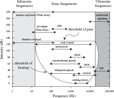
FIGURE 15.1
Tonal quality, or timbre, represents the complex wave pattern that is generated when the overtones of an instrument, voice, etc., are present along with the fundamental frequency. To demonstrate what overtones mean, consider a simple tuning fork that has a resonant frequency of 261.6 Hz (middle C). If you treat the fork as an ideal vibrator, when it is hit, it will vibrate off soundwaves with a frequency of 261.6 Hz. In this case, you have no overtones—you only get one frequency. But now, if you play middle C on a violin, you get an intensely sounding 261.1 Hz, along with a number of other higher, typically less intense frequencies called overtones (or harmonics). The most intense frequency sounded is typically referred to as the fundamental frequency. The overtones of importance have frequencies that are integer multiples of the fundamental frequency (e.g., 2 × 261.1 Hz is the first harmonic, 3 × 261.1 Hz is the second harmonic, and n × 261.1 Hz is the nth harmonic). It is the specific intensity of each overtone within the harmonic spectrum of an instrument, voice, etc., that is largely responsible for giving the instrument, voice, etc. its unique tonal quality. (The reason for an instrument’s unique set of overtones depends on the construction of the instrument.) Figure 15.2a shows a harmonic spectrum (spectral plot) for an oboe that is tuned to middle C—the fundamental frequency.
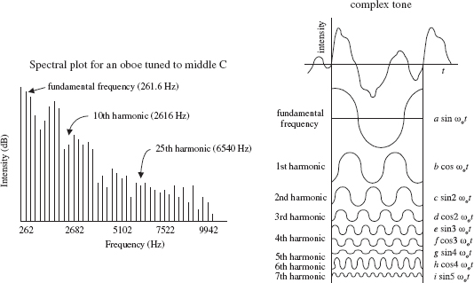
FIGURE 15.2
In theory, you can create the sound from any type of instrument (e.g., violin, tuba, banjo, etc.) by examining the harmonic spectrum of that instrument. To illustrate how this can be done, pretend that you have a number of ideal tuning forks. One fork represents the fundamental frequency; the other forks represent the various overtone frequencies. Using the harmonic spectrum of an instrument as a guide, you can mimic the sound of the instrument by varying the intensity of each “overtone fork.” (In reality, to accurately mimic an instrument, you also must consider rise and decay times of certain overtones—controlling the intensities of the overtones is not enough.) Mathematically, you can express a complex sound as the sum of all its overtones:
Signal = a sin ω0t + b cos ω0t + c sin 2ω0t + d cos 2ω0t + e sin 3ω0t + f cos ω0t + …
The coefficients a, b, c, d, etc., are the intensities of the overtones, and the fundamental frequency f0 = ω0/2π. This expression is referred to as a Fourier series. The coefficients must be calculated from the given waveform or the data from which it is plotted—although an instrument called a harmonic analyzer can automatically compute the coefficients. Figure 15.2b shows a complex sound made up of seven of its harmonics.
The art of synthesizing sounds via electric circuits is fairly complex business. To accurately mimic an instrumental sound, train whistle, bird chirp, etc., you must design circuits that can generate complex waveforms that contain all the overtones and decay and rise time information. For this purpose, special oscillator and modulator circuits are needed.
15.2 Microphones
A microphone converts variations in sound pressure into corresponding variations in electric current. The amplitude of the ac voltage generated by a microphone is proportional to the intensity of the sound, while the frequency of the ac voltage corresponds to the frequency of the sound. (Note that if overtones are present within the sound signal, these overtones also will be present in the electrical signal.) Three commonly used microphones are listed next.
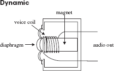
This type of microphone consists of a plastic diaphragm, voice coil, and a permanent magnet. The diaphragm is connected to one end of the voice coil, while the other end of the coil is loosely supported around (or within) the magnet. When an alternating pressure is applied to the diaphragm, the voice coil alternates in response. Since the voice coil is accelerating through the magnet’s magnetic field, an induced voltage is set up across the leads of the voice coil. You can use this voltage to power a very small load, or you can use an amplifier to increase the strength of the signal so as to drive a larger load. Dynamic microphones are extremely rugged, provide smooth and extended frequency response, do not require an external dc source to drive them, perform well over a wide range of temperatures, and have a low impedance output. Some dynamic microphones house internal transformers within their bodies, which give them the ability to have either a high- or low-impedance output—a switch is used to select between the two. Dynamic microphones are widely used in public address, hi-fi, and recording applications.
FIGURE 15.3
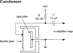
This type of microphone consists of a pair of charged plates that can be forced closer or further apart by variations in air pressure. In effect, the plates act like a sound-sensitive capacitor. One plate is made of a rigid metal that is fixed in place and grounded. The other plate is made of a flexible metal or metal-coiled plastic that is positively charged by means of an external voltage source. A very low-noise, high-impedance amplifier is required to operate this type of microphone and to provide low output impedance. Condenser microphones offer crisp, low-noise sound and are used for high-quality sound recording.
FIGURE 15.4
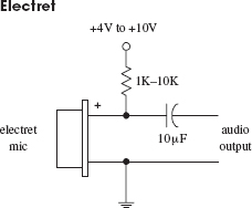
An electret microphone is a variation of the condenser microphone. Instead of requiring an external voltage source to charge the diaphragm, it uses a permanently charged plastic element (electret) placed in parallel with a conductive metal backplate. Most electret microphones have a small FET amplifier built into their cases. This amplifier requires power to operate—typically a voltage between +1.5 and +10 V is needed. This voltage is fed into the microphone through a resistor (1–10 K) (see figure). Electret microphones used to suffer from poor performance, but modern designs can achieve results comparable to those of a condenser microphone.
FIGURE 15.5
15.3 Microphone Specifications
A microphone’s sensitivity represents the ratio of electrical output (voltage) to the intensity of sound input. Sensitivity is often expressed in decibels with respect to a reference sound pressure of 1 dyn/cm2.
The frequency response of a microphone is a measure of the microphone’s ability to convert different acoustical frequencies into ac voltages. For speech, the frequency response of a microphone need only cover a range from around 100 to 3000 Hz. However, for hi-fi applications, the frequency response of the microphone must cover a wider range, from around 20 to 20,000 Hz.
The directivity characteristic of a microphone refers to how well the microphone responds to sound coming from different directions. Omnidirectional microphones respond equally well in all directions, whereas directional microphones respond well only in specific directions.
The impedance of a microphone represents how much the microphone resists the flow of an ac signal. Low-impedance microphones are classified as having an impedance of less than 600 Ω. Medium-impedance microphones range from 600 to 10,000 Ω, whereas high-impedance microphones extend above 10,000 Ω. In modern audio systems, it is desirable to connect a lower-impedance microphone to a higher-impedance input device (e.g., 50-Ω microphone to 600-Ω mixer), but it is undesirable to connect a high-impedance microphone to a low-impedance input. In the first case, not much signal loss will occur, whereas in the second case, a significant amount of signal loss may occur. The standard rule of thumb is to allow the load impedance to be 10 times the source impedance. We’ll take a closer look at impedance matching later on in this chapter.
15.4 Audio Amplifiers
Electrical signals within audio circuits often require amplification to effectively drive other circuit elements or devices. Perhaps the easiest and most efficient way to amplify a signal is to use an op amp. General-purpose op amps such as the 741 will work fine for many noncritical audio applications, but they may cause distortion and other undesirable effects when audio signals get complex. A better choice for audio applications is to use an audio op amp especially designed to handle audio signals. Audio amplifiers have high slew rates, high gain-bandwidth products, high input impedances, low distortion, high voltage/power operation, and very low input noise. There are a number of good op amps produced by a number of different manufacturers. Some high-quality op amps worth mentioning include the AD842, AD847, AD845, AD797, NE5532, NE5534, NE5535, OP-27, LT1115, LM833, OPA2604, OP249, HA5112, LM4562, OPA134, OPA2134, and LT1057.
15.4.1 Inverting Amplifier
The following two circuits act as inverting amplifiers. The gain for both circuits is determined by −R2/R1 (see Chap. 8 for the theory), while the input impedance is approximately equal to R1. The first op amp circuit uses a dual power supply, while the second op amp circuit uses a single power supply.

In both amplifier circuits, C1 acts as an ac coupling capacitor—it acts to pass ac signals while preventing unwanted dc signals from passing from the previous stage. Without C1, dc levels would be present at the op amp’s output, which in turn could lead to amplifier saturation and distortion as the ac portion of the input signal is amplified. C1 also helps prevent low-frequency noise from reaching the amplifier’s input.
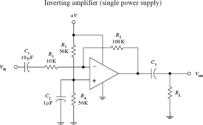
In the single-power-supply circuit, biasing resistors R3 and R4 are needed to prevent the amplifier from clipping during negative swings in the audio input signals. They act to give the op amp’s output a dc level on which the ac signal can safely fluctuate. Setting R3 = R4 sets the dc level of the op amp’s output to 1/2 (+V). For reliable results, the biasing resistors should have resistance values between 10 and 100 k. Now, to prevent passing the dc level onto the next stage, C3 (ac coupling capacitor) must be included. Its value should be equal to 1/(2πfCRL), where RL is the load resistance, and fC is the cutoff frequency. C2 acts as a filtering capacitor used to eliminate power-supply noise from reaching the op amp’s noninverting input.
Notably, many audio op amps are especially designed for single-supply operation—they do not require biasing resistors.
Notably, many audio op amps are especially designed for single-supply operation—they do not require biasing resistors.
FIGURE 15.6
15.4.2 Noninverting Amplifier
The preceding inverting amplifier works fine for many applications, but its input impedance is not incredibly large. To achieve a larger input impedance (useful when bridging a high-impedance source to the input of an amplifier), you can use one of the following noninverting amplifiers. The left amplifier circuit uses a dual power supply, whereas the right amplifier circuit uses a single power supply. The gain for both circuits is equal to R2/R1 + 1.
15.4.3 Digital Amplifiers
Digital power amplifiers are also known as class-D amplifiers or PWM amplifiers. They are extremely efficient and so run quite cool. This makes them ideal for very high-power amplifiers of powers in the hundreds of watts or even the kilowatts range.

FIGURE 15.7 Components R1, C1, R2, and the biasing resistors serve the same function as was seen in the inverting amplifier circuits. The noninverting input offers an exceptionally high input impedance and can be matched to the source impedance more readily by adjusting C2 and R3 (dual-supply circuit) or R4 (single-supply circuit). The input impedance is approximately equal to R3 (dual-supply circuit) or R4 (single-supply circuit).
Figure 15.8 shows the block diagram for a class-D amplifier. The input signal is converted into a PWM signal by comparing it with a triangle wave. This is a very neat trick. As the triangle wave rises, at some point, it will become greater than the signal voltage. If the signal voltage is high, this will take longer; if the voltage is low, it will happen sooner. In this way, the pulse length produced will be proportional to the instantaneous input voltage.
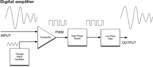
FIGURE 15.8
Figure 15.9 shows the result of simulating the comparator with a triangle waveform of 10 kHz sampling a sine wave input signal at 1 kHz. The squarewave is the PWM output.
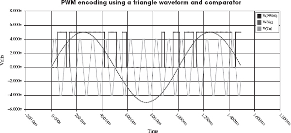
FIGURE 15.9
We have digitized our audio signal. It is now just on or off. So we can use that to switch as high a current as we like, using big MOSFETs in a complementary arrangement or some other switching transistor. This high-power PWM signal will be conveying the right energy at the right time, but it is being carried in the high-frequency switching squarewave. This needs low-pass filtering to remove this carrier, leaving just the original signal in amplified form.
The quality of digital amplifiers can be very variable, but their efficiency makes them an attractive proposition. There are a number of ICs available that either encapsulate the whole amplifier in one device or provide outputs suitable for driving a complementary pair of MOSFETs. A couple devices to look at are the NCP2704 and LX1720.
15.4.4 Reducing Hum in Audio Amplifiers
If your project includes an audio amplifier that you are designing yourself, then you need to consider hum. Domestic power lines and devices will easily induce an annoying 60 Hz hum in an audio amplifier. Some of this signal can arrive through the amplifier’s power supply. Hence, design of power supplies for hi-fi amplifiers is almost as important as the designs for the amplifiers themselves. The main thing is to add as much smoothing capacitance to the power supply as possible.
Other 60 Hz signals will arrive in your audio amplifier circuit by mutual induction with wires and tracks on your PCB. You should make sure that you keep all PCB tracks and wires as short as possible. Wires should also be screened with the screening layer grounded.
15.5 Preamplifiers
In most audio applications, the term preamplifier refers to a control amplifier that is used to control features such as input selection, level control, gain, and impedance levels. Here are a few simple microphone preamplifier circuits to get you started. (Note that “high Z” refers to a microphone with a high input impedance—one that is greater than ~600 Ω.)
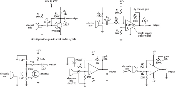
FIGURE 15.10
Audio mixers are basically summing amplifiers—they add a number of different input signals together to form a single superimposed output signal. The two circuits below are simple audio mixer circuits. The left circuit uses a common-emitter amplifier as the summing element, while the right circuit uses an op amp. The potentiometers are used as independent input volume controls.
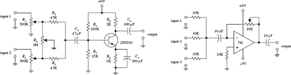
FIGURE 15.11
15.7 A Note on Impedance Matching
Is matching impedances between audio devices necessary? Not any more, at least when it comes to connecting a low-impedance source to a high-impedance load. In the era when vacuum-tube amplifiers were the standard, it was important to match impedances to achieve maximum power transfer between two devices. Impedance matching reduced the number of vacuum-tube amplifiers needed in circuit design (e.g., the number of vacuum-tube amplifiers needed along a telephone transmission line). However, with the advent of the transistor, more efficient amplifiers were created. For these new amplifiers, what was important—and still is important—was maximum voltage transfer, not maximum power transfer. (Think of an op amp with its extremely high input impedance and low output impedance. To initiate a large-output- current response from an op amp, practically no input current is required into its input leads.) For maximum voltage transfer to occur, it was found that the destination device (called the load) should have an impedance of at least 10 times that of the sending device (called the source). This condition is referred to as bridging. (Without applying the bridging rule, if two audio devices with the same impedances are joined, you would see around a 6 dB worth of attenuation loss in the transmitted signal.) Bridging is the most common circuit configuration used when connecting modern audio devices. It is also applied to most other electronic source-load connections, with the exception of certain radiofrequency circuits where matching impedance is usually desired and in cases where the signal being transmitted is a current rather than a voltage. If the transmitted signal is a current, the source impedance should be larger than the load impedance.
Now, if you consider a high-impedance source connected to a low-impedance load (e.g., a high-impedance microphone connected to a low-impedance mixer), voltage transfer can result in significant signal loss. The amount of signal loss in this case would be equal to
As a rule of thumb, a loss of 6 dB or less is acceptable for most applications.
15.8 Speakers
Speakers convert electrical signals into audible signals. The most popular speaker used today is the dynamic speaker. The dynamic speaker operates on the same basic principle as a dynamic microphone. When a fluctuating current is applied through a moving coil (voice coil) that surrounds a magnet (or that is surrounded by a magnet), the coil is forced back and forth. A large paper cone attached to the coil responds to the back-and- forth motion by “drumming off” sound waves.
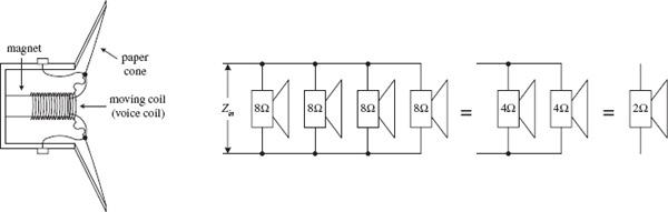
FIGURE 15.12
Every speaker is given a nominal impedance Z that represents the average impedance across its leads. (In reality, a speaker’s impedance varies slightly with frequency, above and below the nominal level.) In terms of applications, you can treat the speaker like a simple resistive load of impedance Z. For example, if you attach an 8-Ω speaker to an amplifier’s output, the amplifier will treat the speaker as an 8-Ω load. The amount of current drawn from the amplifier will be I = Vout/Zspeaker. However, if you replace the 8-Ω speaker with a 4-Ω speaker, the current drawn from the amplifier will double.
Driving two 8-Ω speakers in parallel is equivalent to driving a 4-Ω speaker. Driving two 4-Ω speakers in parallel is equivalent to driving a 2-Ω speaker. By using high-power resistors, it is possible to change the overall impedance sensed by the amplifier. For example, by placing a 4-Ω resistor in series with a 4-Ω speaker, you can create a load impedance of 8 Ω. However, using a series resistor to increase the impedance may hurt the sound quality. There are speaker-matching transformers that can change from 4 to 8 Ω, but a high-quality transformer like this can cost as much as a new speaker and can add slight frequency response and dynamic range errors.
Another important characteristic of a speaker is its frequency response. The frequency response represents the range over which a speaker can effectively vibrate off audio signals. Speakers that are designed to respond to low frequencies (typically less than 200 Hz) are referred to as woofers. Midrange speakers are designed to handle frequencies typically between 500 and around 3000 Hz. A tweeter is a special type of speaker (typically dome or horn type) that can handle frequencies above midrange. Some speakers are designed as full-range units that are capable of reproducing frequencies from around 100 to 15,000 Hz. A full-range speaker’s sound quality tends to be inferior to a speaker system that incorporates a woofer, midrange, and tweeter speaker all together.
15.9 Crossover Networks
To design a decent speaker system, it would be best to incorporate a woofer, midrange speaker, and tweeter together so that you get good sound response over the entire audio spectrum (20 to 20,000 Hz). However, simply connecting these speakers in parallel will not work because each speaker will be receiving frequencies outside its natural frequency-response range. What you need is a filter network that can divert high-frequency signals to the tweeter, low-frequency signals to the woofer, and midrange-frequency signals to the midrange speaker. The filter network that is used for this sort of application is called a crossover network.
There are two types of crossovers: passive or active. Passive crossover networks consist of passive filter elements (e.g., capacitors, resistors, inductors) that are placed between the power amplifier and the speaker—they are placed inside the speaker cabinet. Passive crossover networks are cheap to make, easy to make foolproof, and can be tailored for a specific speaker. However, they are nonadjustable and always use up some amplifier power. Active crossover networks consist of a set of active filters (op amp filters) that are placed before the amplifier section. The fact that active crossover networks come before the power amplifier section makes it easier to manipulate the signal because the signal is still tiny (not amplified). Also, a single active crossover network can be used to control a number of different amplifier-speaker combinations at the same time. Since active crossover networks use active filters, the audio signal will not suffer as much attenuation loss as it would if it were applied through a passive crossover network.
Figure 15.13 shows a simple passive crossover network used to drive a three-speaker system. The graph shows typical frequency-response curves for each speaker. To produce an overall flat response from the system, you use a low-pass, bandpass, and high-pass filter. C1 and Rt form the low-pass filter, L1, C1, and Rm form the bandpass filter, and L2 and Rw form the low-pass filter (Rt, Rm, and Rw are the nominal impedances of the tweeter, midrange, and woofer speakers).

FIGURE 15.13
To determine the component values needed to get the desired response, use the following: C1 = 1/(2πf2Rt), L1 = Rm/(2πf2), C2 = 1/(2πf1Rm), and L2 = Rw/2πf1, where f1 and f2 represent the 3-dB points shown in the graph. Usually, passive crossover networks are a bit more sophisticated than the one presented here. They often incorporate higher-order filters along with additional elements, such as an impedance compensation network, attenuation network, series notch filter, etc., all of which are used to achieve a flatter overall response.
Here is a more practical passive crossover network (crossover frequency 1.8 kHz) used to drive a two-speaker system consisting of an 8-Ω tweeter and an 8-Ω woofer. An 18 × 12 × 8 in fiberboard box acts as a good resonant cavity for this system.
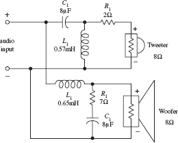
FIGURE 15.14
The following is an active crossover network that is used to drive a two-speaker system that has a crossover frequency (3-dB point) around 600 Hz and 18 dB per octave response. A LF356 high-performance op amp is used as the active element. Remember that for active filters the output signals must be amplified before they are applied to the speaker inputs.
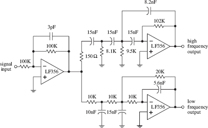
FIGURE 15.15
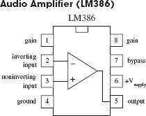

The LM386 audio amplifier is designed primarily for low-power applications. A +4- to +15-V supply voltage is used to power the IC. Unlike a traditional op amp, such as the 741, the 386’s gain is internally fixed to 20. However, it is possible to increase the gain to 200 by connecting a resistor-capacitor network between pins 1 and 8. The 386’s inputs are referenced to ground, while internal circuitry automatically biases the output signal to one-half the supply voltage. This audio amplifier is designed to drive an 8-Ω speaker.
FIGURE 15.16
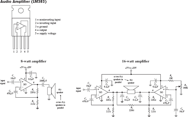
The LM383 is a power amplifier designed to drive a 4-Ω speaker or two 8-Ω speakers in parallel. It contains thermal shutdown circuitry to protect itself from excessive loading. A heat sink is required to avoid shutdown at levels below the maximum power output.
FIGURE 15.17
There are a number of unique audible-signal devices that are used as simple warning signal indicators. Some of these devices produce a continuous tone, others produce intermittent tones, and still others are capable of generating a number of different frequency tones, along with various periodic on/off cycling characteristics. Audible-signal devices come in both dc and ac types and in various shapes and sizes. Some of these devices are extremely small—no bigger than a dime. A good electronics catalog will provide a listing of audio-signal devices, along with their size, sound type, dB ratings, voltage ratings, and current-drain specifications.
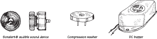
FIGURE 15.18
15.12 Miscellaneous Audio Circuits

FIGURE 15.19
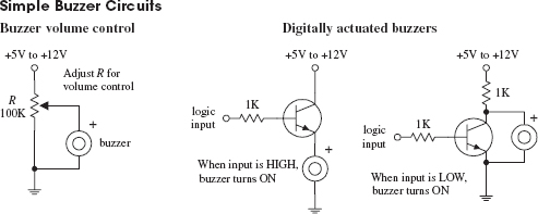

FIGURE 15.21
FIGURE 15.22
..................Content has been hidden....................
You can't read the all page of ebook, please click here login for view all page.