Sensors
Sensors are devices that measure a physical property, such as temperature, humidity, stress, and so on. As this is an electronics book, we are concerned with converting such measurements into electrical signals. We have also stretched the definition of a sensor a little to include things such as global positioning systems (GPSs) that locate your position in space.
Many sensors will provide an output signal that is simply a voltage proportional to the property being measured. Others are digital devices that provide digital data about the property. In both cases, these measurements will often be the input to a microcontroller.
6.1 General Principals
Before we look at some of the vast array of sensors that are available, we will cover some of the general principles that underpin all sensing.
6.1.1 Precision, Accuracy, and Resolution
When looking at a sensor, it is important to understand the difference between precision and accuracy, particularly as precision often gives a misleading impression of the accuracy of the sensor. A classic example of this is with digital weighting scales. These may confidently tell you that you weigh 85.7 kilograms when you actually weigh 92.1 kilograms. This is only an error of 10 percent or so, and may not matter if you always use the same scales, but as an absolute measurement, it might be well off the mark.
So precision is a matter of the number of digits reported by the sensor. For an analog sensor, the readings are continuous.
When it comes to digital sensors, there will be a number of bits of resolution. That might be 8 bits (1 in 256), 12 bits (1 in 4096), or higher; that is, the reading is no longer continuous, but has been quantized.
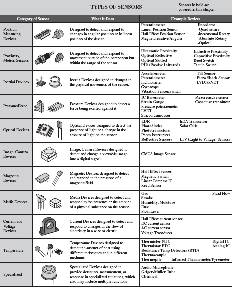
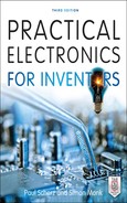
FIGURE 6.1 Sensor types
6.1.2 The Observer Effect
The observer effect states that the act of observing a property changes it. This is the case in a car tire, for example. When you measure the pressure with a conventional tire gauge, you will let a little of the air out, thus changing the pressure that you are measuring. For most sensors, this change will have a negligible effect, but it is something worth keeping at the back of your mind when deciding whether you are getting a true reading.
6.1.3 Calibration
If your invention is a low-cost consumer item that will be mass-produced, then it will be much cheaper and easier to produce if there is no calibration to do. In fact, individual calibration to take differences in individual sensors into account is likely to be prohibitively expensive.

FIGURE 6.2 Sensors
If, on the other hand, your invention is specialized, high-value equipment, then individual calibration of sensors is possible.
The principal of calibration is the same whatever property the sensor measures. The idea is that you take a number of readings from the sensor of unknown accuracy while the sensor is measuring a standard value of known accuracy. So, to calibrate a temperature sensor, your accurate standard might be boiling distilled water at 100°C, or more likely, the temperature in a highly accurate oven constructed for the purpose of calibrating the sensor. This oven will itself need to have been calibrated against an even more accurate standard.
When you have discovered the degree to which your sensor deviates from the standard, then you can compensate for it in some way. Since the sensor will almost certainly be supplying information to a microcontroller, a common way to make the calibration is to change the values in a lookup table. This table contains accurate values against raw values. For example, the raw value straight from a 12-bit analog-to-digital converter is a number between 0 and 1023. These numbers, perhaps in increments of 5, might be the left-hand side of the table, with the right-hand side of the table containing the equivalent temperature as a decimal in degrees Celsius. Interpolation can be used in the gaps between the raw readings by assuming that the small segment of the curve is linear (see Fig. 6.3).

FIGURE 6.3 Actual reading against raw value for a fictional sensor
Some IC sensors are actually calibrated individually during the manufacturing process, with the values for the lookup table being written into the read-only memory (ROM) of the sensor. This allows accurate sensing at low cost.
6.2 Temperature
Temperature sensors are one of the most common types of sensors. Computers and many types of equipment will sense their own temperature to prevent overheating. In addition, as well as electronic thermometers, there are thermostats that keep temperature constant by controlling the power to a load, usually just turning it on and off. Figure 6.4 shows a variety of temperature sensors.
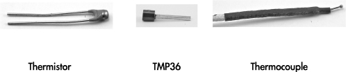
FIGURE 6.4 Temperature sensors
The term “thermistor” is a combination of the words “thermal” and “resistor.” A thermistor is a resistor whose resistance changes markedly with temperature. Thermistors come in two flavors: negative temperature coefficient (NTC) and positive temperature coefficient (PTC). An NTC thermistor’s resistance will decrease with increasing temperature, and a PTC thermistor will behave the opposite way, with the resistance increasing as temperature increases. The NTC is the more common type.
The relationship between temperature and resistance in a thermocouple is not a linear one. Even over relatively short temperature ranges—say 0 to 100°C, a linear approximation will introduce considerable errors (see Fig. 6.5).
FIGURE 6.5 Resistance against temperature for an NTC thermistor
The Steinhart-Hart equation is a third-order approximation used to determine the temperature as a function of the thermistor’s resistance. It works for both NTC and PTC devices. It is normally stated as:
(6.1)
T is the temperature in Kelvin; R is the resistance of the thermistor; and A, B, and C are constants specific to that thermistor. The manufacturer of a thermistor will give all three constant values.
An alternative and more common model for this relationship uses a single parameter (Beta) and assumes constants of T0 and R0, where T0 is usually 25°C and R0 is the resistance of the thermistor at that temperature.
Using this equation, the temperature can be approximated to:
(6.2)

(6.3)
As well as providing Beta, T0, and R0, the data sheet will also specify a temperature range and accuracy.
To use a thermistor as a thermometer for input to a microcontroller, a voltage is required that can be measured by the analog-to-digital converter of the microcontroller. Figure 6.6 shows a typical arrangement using a potential divider with a fixed-value resistor of the same value as R0.
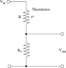
FIGURE 6.6 Using a thermistor as a thermometer
If we place a NTC thermistor at the top of the potential divider, then as the temperature of the thermistor increases, its resistance falls and Vout rises.
Looking at Fig. 6.6:
(6.4)
Combining Formula 6.3 with Formula 6.4, we have:
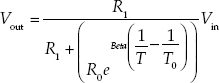
(6.5)
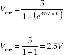
Example 1: Using a potential divider as shown in Fig. 6.3 with a fixed resistor of 4.7 kΩ and an NTC thermistor with a T0 of 25°C, an R0 of 4.7 kΩ, and a Beta of 3977, what is the formula for calculating Vout?
Answer 1: Just substituting the values into the equation, we get:
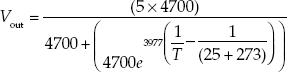
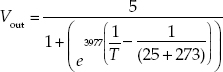
Note that 273 is added to the temperature in °C to give a temperature in °K.
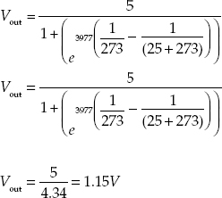
Example 2: Using the same setup as Example 1, what is Vout at 25°C?
Answer 2: In one way, this is a trick question, since by definition the thermistor’s resistance at 25°C will be 4.7 kΩ, so the voltage will be 2.5 V. However, we can apply the formula as a sanity check:
Example 3: Using the same setup as Examples 1 and 2, what is Vout at 0°C?
Answer 3:
6.2.2 Thermocouples
While thermistors are good for measuring relatively small ranges in temperature—typically –40 to +125°C, for much higher temperatures and temperature ranges, thermocouples are used (see Fig. 6.7).
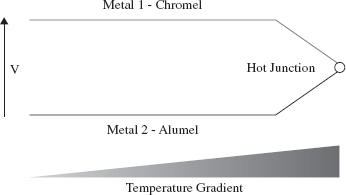
FIGURE 6.7 Thermocouples
Any conductor subjected to a thermal gradient will experience something called the Seebeck effect; that is, it will generate a small voltage. The magnitude of this voltage is dependent on the type of metal, so if two different metals are joined, the temperature of that junction can be measured by measuring the voltage across the metal leads, at the far end from the junction. It is also necessary to measure the temperature at the other end of the thermocouple leads (often using a thermistor, since this will probably be at room temperature). This second temperature is called the “cold-junction” temperature.
Lookup tables are often used to calculate the absolute temperature at the junction, based on the voltage and the cold-junction temperature, as the relationship is not completely linear and needs a fifth-order polynomial to model it accurately. Manufacturer’s data sheets for thermocouples will normally contain large tables for calculating the temperature.
The most commonly used metals for a thermocouple are the alloys chromel (90 percent nickel and 10 percent chromium) and alumel (95 percent nickel, 2 percent manganese, 2 percent aluminum, and 1 percent silicon). A thermocouple made with these materials will typically be able to measure temperatures over the range –200°C to +1350°C. The sensitivity is 41 μV / °C for these metals.
6.2.3 Resistive Temperature Detectors
Resistive temperature detectors (RTDs) are perhaps the simplest temperature sensors to understand. Like thermistors, RTDs rely on their resistance changing with temperature. However, rather than use a special material that is sensitive to temperature changes (like a thermistor), they simply use a coil of wire (normally platinum) around a glass or ceramic core. The resistance of the core is often contrived to be 100 Ω at 0°C.
RTDs are much less sensitive than thermistors and can therefore be used over a much wider range of temperatures. The resistance of platinum changes in a relatively linear manner, and can be assumed to be linear for a range of 100°C or so. For the range 0 to 100°C, the resistance of a platinum RTD will vary by 0.003925 Ω/Ω/°C.
So, a 100 Ω (at 0°C) platinum RTD will, at a temperature of 100°C, have a resistance of:
100Ω + 100°C × 100 Ω × 0.003925 Ω/Ω/°C = 139.25 Ω
The first 100 Ω in the equation above is for the base resistance of the RTD at 0°C.
This can be arranged in a potential divider in the same way as a thermistor.
6.2.4 Analog Output Thermometer ICs
An alternative to using a thermistor and fixed-value resistor in a potential divider arrangement is to use a special-purpose temperature measurement IC.
Devices such as the TMP36 come in a three-pin package and are used as shown in Fig. 6.8.

FIGURE 6.8 TMP36 temperature sensor
Unlike a thermistor, the sensor’s output voltage is almost linear at 10 mV / °C for a temperature range of –40 to +125°C. The accuracy is only ±2°C over the temperature range.
The temperature in °C is simply calculated from Vout using the formula:
T = 100Vout – 50
The constant 50 is specified in the data sheet for the TMP36.
These devices are considerably more expensive than thermistors and series resistors, but they are very easy and convenient to use.
6.2.5 Digital Thermometer ICs
An even higher technology approach to temperature measurement is to use a digital thermometer IC. These devices have a serial interface for use by microcontrollers.
A typical digital thermometer IC is the DS18B20. It uses a serial bus standard called 1-Wire that can allow multiple sensors to share the same data line (see Fig. 6.9).
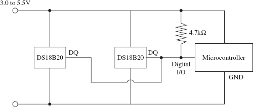
FIGURE 6.9 DS18B20 temperature sensor IC
These devices are more accurate than the linear devices such as the TMP36. The digital thermometer IC has a stated accuracy of ±0.5°C and a temperature range of –55°C to +125°C.
Since digital thermometer ICs transmit their data digitally, they are very suitable for remote sensing, as lead length and electrical interference will have less effect than with an analog device. In fact, they will either work accurately or not at all in an electrically noisy environment.
Digital thermometer ICs can also be configured to work in “parasitic” power mode, where they harvest power from the data line, allowing them to be connected with just two wires. The GND and positive supply to the DS18B20 are both grounded, and the microcontroller must control a MOSFET transistor that pulls the data line up to the supply voltage under strict timing conditions.
Chapter 13 contains more information about using the 1-Wire interface with microcontrollers.
6.2.6 Infrared Thermometers/Pyrometers
If you have been to the doctor recently and have had your temperature taken, you will probably have seen an infrared thermometer that is placed near your ear and measures the temperature just on the inside surface of the ear without any actual contact. The ear is chosen because it is effectively a hole into the body that is free from the influence of external radiation, so that the back surface of the ear acts as a “black-body” radiator.
Pyrometers, or more specifically, broadband pyrometers, measure the radiation intensity, which has dimensions of energy per second per unit of area and use the Stefan-Boltzmann law to determine the temperature:
j* = σT4
The radiation intensity (j*) is proportional to the fourth power of the temperature, where σ is the Stefan-Boltzmann constant (5.6704 × 10⁻⁸ Js–1m–2K–4).
These devices use an infrared sensor such as the MLX90614 coupled with optics that focus the infrared radiation from the subject onto the sensor. When used for other measurement applications, the infrared thermometer will often have a low-power laser align with the sensor so that it can be aimed to take spot readings of temperature.
Devices such as the MLX90614 are more than just a sensor, containing a low-noise amplifier, high-precision analog-to-digital converter, and all the associated electronics to produce a digital output.
As with other IC sensors, the advantages of including all the electronics in the same package as the sensor itself are the reduction of noise and simplicity of interfacing.
Other sensors are available for high temperatures, such as those found in industrial furnaces, and the term “pyrometer,” with its overtones of fire, is usually reserved for such high-temperature applications.
6.2.7 Summary
Table 6.1 shows a number of temperature sensors and their characteristics.
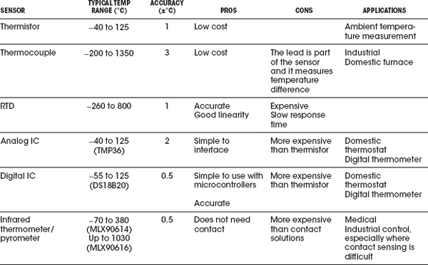
The figures for accuracy in Table 6.1 are somewhat arbitrary, as for most sensors, high accuracy can be obtained by individual calibration. It is also the accuracy of the overall system—including the electronics that use the sensor value—that counts. The figures assume the use of off-the-shelf components using data sheet parameters without any individual calibration and are meant as an indication of the likely accuracy of measurement that can be achieved with such a sensor.
6.3 Proximity and Touch
This section deals with detecting objects or measuring their distance from the sensor. Figure 6.10 shows a selection of such sensors
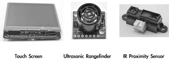
FIGURE 6.10 Proximity and touch sensors
6.3.1 Touch Screens
Touch screens are commonly used in cellular phones and tablet computers. There are many different technologies used in touch screens. The most commonly used are resistive touch screens.
Resistive touch screens are one of the older and more readily used touch screen technologies. They rely on a transparent sheet on top of the display. This sheet is flexible and also conductive. Figure 6.11 shows a typical arrangement for a four-wire resistive touch screen.
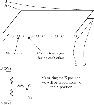
FIGURE 6.11 Resistive touch screen
Both the top and bottom surfaces are coated with a conductive layer. Insulating dots are evenly sprayed onto the rigid bottom surface to keep the layers apart, except when they are pressed together.
To determine the X position of a touch, A is set to 0 V and B to 5 V, establishing a voltage gradient across the top surface. The voltage measured at C, or for that matter D, will be proportional to the X position. This is converted into coordinates using an analog-to-digital converter.
The conductive layer acts just like a potentiometer with C as the slider. If the device measuring the voltage at C has a very high input impedance, then the resistance of the track from the surface to the terminal C can be ignored. Most microcontrollers will have an analog-to-digital converter with a high input resistance, typically several MΩ. So, the voltage at C will be between 0 and 5 V in direct proportion to the distance from A of the touch.
When it comes to reading the Y position, some crafty footwork has to take place. Now C will be set to 0V, D to 5V, and the voltage measured at A or B.
All this processing will be carried out by either a special-purpose controller chip or a microcontroller.
6.3.2 Ultrasonic Distance
Ultrasonic distance-measuring devices are much loved by the developers of hobby robots. They are also found in commercial equivalents to the tape measure.
These devices send out a pulse of ultrasound and time how long it takes for the reflection to come back. A simple calculation involving the speed of sound will determine the distance to the object (see Fig. 6.12).

FIGURE 6.12 Ultrasonic distance measurement
These devices have a measurement range of up to around 5 meters (15 ft), but this depends very much on the size and sound reflecting properties of the object. They also suffer limits of accuracy due to variations in the speed of sound, which is dependent on many factors, including atmospheric pressure, humidity, and temperature. For example, at 0°C, the speed of sound in dry air is 331 meters/seconds, but this rises to 346 meters/second at 25°C—a difference of 4.5 percent.
Sometimes separate transducers are used for sending and receiving the pulses of ultrasound, and sometimes a single transducer is used in both roles.
Some devices rely on a microcontroller to initiate the pulse and time the echo. Other, more expensive, devices will have their own digital processing that generates an output that can be read from a microcontroller as one of the following:
• An analog output voltage proportional to the distance
• Serial data
• A train of varying pulse lengths dependent on the distance
In some cases, all three outputs are provided, such as with the SparkFun device SKU: SEN-00639.
Example: Assuming that in dry air at 20°C, the speed of sound is 340 meters/second, if the time period between a pulse of ultrasound being sent is 10 milliseconds, how far away is the reflecting object?
Answer: distance = velocity × time = 340 × 0.01 = 3.4m
However, that is the distance for the entire round-trip, so the actual distance to the object is half of that, or 1.7 meters.
6.3.3 Optical Distance
Another useful device for measuring distance at close range is the infrared optical sensor (see Fig. 6.13). This type of device uses the amount of reflection of a modulated infrared pulse to determine the distance to the object. The Sharp GP2Y0A21YK (SparkFun SKU: SEN-00242) is a typical sensor of this type.

FIGURE 6.13 Optical distance measurement
Infrared optical sensors are used for closer range measurements than the ultrasonic devices and produce an analog output. This is not linear or particularly accurate, so these devices are most useful for simple proximity detection rather than actual measurement.
At close range, the measurements become ambiguous, as shown in the distance/output voltage plot of Fig. 6.14. Therefore, they are usually mounted recessed so that no object can get closer than the ambiguous distance, which is about 5 cm for the sensor in Fig. 6.14.

FIGURE 6.14 Output against distance for a Sharp GP2Y0A21YK
When this type of sensor is used with a microcontroller, a lookup table is used to convert the measured voltage to a distance reading.
In some circumstances, you just need to know whether or not something is present. This can be detected with a slotted optical sensor, where the infrared source and sensor are aligned with a slot in between. When the beam is broken, the object is detected.
Capacitive sensors are frequently used as proximity or touch sensors as a replacement for mechanical push switches. They sense conductors and therefore are ideal for sensing proximity of a hand or finger.
There are various different approaches to capacitive sensing, but they all follow the basic principals shown in Fig. 6.15.
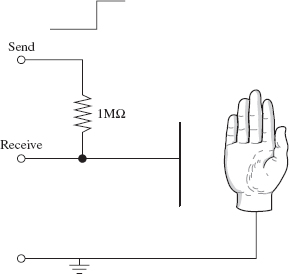
FIGURE 6.15 Capacitive sensing
In this case, the sensing is accomplished using two general-purpose input/output (GPIO) pins of a microcontroller. The Send pin is configured as an output, and the Receive pin as an input. A single fixed resistor between the two pins forms one half of an RC arrangement, with the capacitor formed by the object being sensed and a sensor plate forming the other half of the capacitor.
When a hand moves close to the plate, the capacitance increases. This is sensed as the control software toggles the state of the Send pin and times how long it takes for the Receive pin to catch up with the changed state. In this way, it effectively measures the capacitance and hence the proximity of the object being sensed. The longer it takes for the Receive pin to change to the same state as the Send pin, the closer the object is to the plate.
This type of sensing has the advantages that it requires very little special hardware and can sense through glass, plastic, and other insulators. More advanced versions of this approach can sense in two dimensions to make a capacitative touch screen.
6.3.5 Summary
Table 6.2 compares the relative merits of the different types of distance sensors.

Another type of sensor that is used in industrial settings is the inductive sensor. This is in essence a mini-metal detector.
Proximity of a magnet can also be detected using magnetic sensors such as Hall effect sensors (discussed in Section 6.6.3) and even the humble read switch, which consists of a pair of contacts in a glass envelope that close when near a magnet.
6.4 Movement, Force, and Pressure
Many different types of sensors can tell us about how things are moving. This has become a common occurrence in smartphones, where an accelerometer is used to detect the orientation of the device for automatic switching of the screen between landscape and portrait format, as well as for game playing. Figure 6.16 shows a variety of different movement-detecting devices.

FIGURE 6.16 Movement sensors
6.4.1 Passive Infrared
Passive infrared (PIR) detectors are most commonly used in intruder alarms. They detect changes in infrared heat. Because they require a plastic lens, they are usually sold as a detector module on a printed circuit board.
More advanced movement detectors will have multiple detectors that respond to a rapid change in the level of infrared heat. When this is detected, the module may activate a relay, or in some modules, switch a transistor with an open collector arrangement.
Figure 6.17 shows how to use an open collector device such as the PIR sensor from SparkFun (SKU: SEN-08630) to give a digital output.

FIGURE 6.17 Using a passive infrared sensor
6.4.2 Acceleration
The ready use of accelerometers in cellular phones has led to them becoming a low-cost and readily available component. The most common of these use a technology called microelectromechanical systems (MEMS). The basic principal for these devices is to measure the position of a mass attached to a spring that stretches under acceleration (see Fig. 6.18). The neat trick is that all of this is fabricated onto an IC.
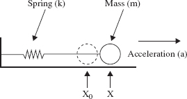
FIGURE 6.18 Mass and spring accelerometer
This arrangement is basically the same as a spring balance of the sort favored by fishermen and travelers worried about exceeding their baggage allowance. In fact, turning it through 90 degrees, you would be measuring the gravitational constant whose units are those of an acceleration. This is how an accelerometer can determine its orientation on the vertical axis.
The force acting on the mass due to the acceleration is:
F = k (x – x0) = m a
Since the manufacturer will know k and m, we just need to be able to measure the displacement of the mass m. Measuring this movement often uses the capacitive effect of the mass, in relation to one or two plates. A common arrangement is for the mass to move between two plates making a capacitive divider (see Fig. 6.19 and Section 2.23.14 in Chap. 2).

FIGURE 6.19 Measuring the offset of the mass
If the mass, shown as a rectangle in between two plates in Fig. 6.19, is halfway between the two plates A and C, then the capacitance between A and B and between B and C will be equal. An acceleration to the left of the diagram will move the weight to the right, changing the ratio of the capacitance.
Most accelerometers come in a little IC package that not only includes three accelerometers—one for each dimension—but also all the necessary electronics, analog-to-digital converters, and digital electronics to provide serial communication of the data back to a microcontroller using an I2C serial interface.
A much used low-cost accelerometer is the MMA8452Q (SparkFun SKU: COM-10953).
6.4.3 Rotation
Measuring rotation can be as simple as using a potentiometer as a voltage divider, where the voltage at the slider is proportional to the angle of rotation (see Fig. 6.20). However, the potentiometer will not measure a full 360 degrees, and it has stops at both ends of the track that prevent it from turning all the way around.

FIGURE 6.20 Measuring rotation with a potentiometer
A more flexible alternative to the potentiometer is the quadrature encoder. This type of device rotates without any stops, so you can just keep turning it. These are often used as an alternative to potentiometers in electrical appliances. They actually just measure steps to the left or steps to the right, rather than the absolute position.
A quadrature encoder is really just a pair of concentric tracks that each has a contact. They act as a pair of switches producing pulses as the shaft is rotated (see Fig. 6.21).

FIGURE 6.21 Outputs from a quadrature encoder
The transitions of A and B are used to determine the direction in which the shaft is being rotated. For example, a clockwise rotation would be read as going from phase 1 to 4 and a counterclockwise from 4 down to 1.
Clockwise (AB): LH HL HH HL
Counterclockwise (AB): HL HH LH LL
Quadrature encoders come in various resolutions. Low-cost ones may have only 12 pulses per revolution. Better-quality devices can have up to 200 pulses per revolution and be designed for high-speed operation of up to 30,000 rpm. Such devices will use optical sensors rather than contacts.
A variation on the quadrature encoders that measure relative rotation are absolute rotary encoders. This type of device is essentially a rotary switch with a number of tracks that then indicate the angle by providing a binary output.
Rather than count in “normal” binary, the binary numbers for each position are arranged so that only one bit changes between one position of the switch and the next. This type of encoding is called a Gray code. For example, the 3-bit Gray code looks like this: 000, 001, 011, 010, 110, 111, 101, 100.
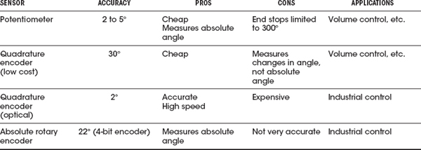
Table 6.3 shows some of the pros and cons of rotation sensors.
TABLE 6.3 Rotation Sensors
6.4.4 Flow
The simplest sensors for measuring flow are variations on some kind of paddle wheel or turbine that is placed in the flow and spins at a speed proportional to the flow. The problem of measuring the rate of rotation remains. An anemometer that measures the wind speed is a typical example of this (see Fig. 6.22).
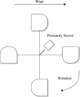
FIGURE 6.22 A cup anemometer
The wind will cause the arrangement of cups to spin at a rate of rotation proportional to the wind strength. Some fixed point on the cup assembly passes close to a proximity sensor that produces a pulse for each full rotation. In this way, you get a stream of pulses at a frequency proportional to the wind speed. Measuring the speed is then just a matter of using a microcontroller to count the number of pulses in a given period of time.
The proximity sensor may be a fixed magnet on the cup assembly and a magnetic sensor such as the Hall effect sensor (described in Section 6.6.3), or may be an optical sensor where a beam is interrupted.
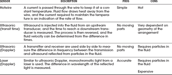
Various types of fluid flow sensors are summarized in Table 6.4.
TABLE 6.4 Flow Sensors
6.4.5 Force
Force can be sensed using a force-sensitive resistor. These devices operate in a similar manner to a resistive touch screen. They are two layers, with conducting tracks and a microdot insulating layer, but the harder you press, the more of the top conductor comes into contact with the bottom conductor and the lower the resistance. These devices are not usually very accurate.
Strain gauges operate on the principal of deforming the geometry of a resistor as it is put under tension or compression (see Fig. 6.23).

FIGURE 6.23 Strain gauge
For a more accurate sensing of force, a load cell is used. This arranges two or more strain gauges bonded onto a deformable metal block. They will often also include temperature compensation.
6.4.6 Tilt
Although an accelerometer can be used to measure the angle of tilt, or just detect tilt from the horizontal, if all that is required is to know that the sensor has tilted from the horizontal, then a simpler sensor can be used. The simplest of these use a small metal ball in a case, which sits on contacts when horizontal but rolls off when the device is tipped.
6.4.7 Vibration and Mechanical Shock
Piezoelectric materials are good for detecting shock and vibration. The vibration sensor in Fig. 6.16 uses a small weight (just a rivet) on the end of a flexible strip of piezoelectric material. When the weight wobbles due to vibration, a voltage is generated across the terminals. The output of these voltages will drift, so for practical use, place a 10 MΩ resistor in parallel with them. This same approach will work for detecting mechanical shock.
6.4.8 Pressure
Unless you plan to work in process control or build a weather station, sensing pressure is unlikely to be something that you will need to do. Except for when you have very particular sensing requirements, the solution is nearly always to buy a digital sensor on a chip, such as the two listed in Table 6.5.
TABLE 6.5 Pressure Sensors

Other types of pressure sensors are on a larger scale, usually based on traditional pressure measurement, such as bellows or a Bourdon tube. These create a physical displacement that is then measured by one of the techniques discussed earlier, such as a potentiometer, a strain gauge, or capacitative position sensing like that used in an IC accelerometer.
There are many sensors available for detecting chemicals of various kinds—far too many to list here. The selection shown in Fig. 6.24 illustrates a range of the sensors available, and we’ll look at their principals of operation in the following sections.

FIGURE 6.24 Chemical sensors
6.5.1 Smoke
Domestic smoke detectors are (or should be) a feature of every home. The most common devices are actually quite sophisticated in their sensing (see Fig. 6.25).
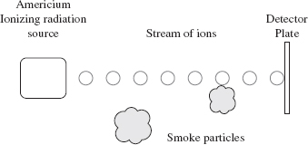
FIGURE 6.25 An ionizing smoke detector
They use a radioisotope (Americium) that generates a stream of ionized particles in a chamber that is open to the air. This allows a small current to flow between the metal casing of the radiation source and a detecting plate at the far side of the chamber.
If smoke particles enter the chamber—even microscopic particles—they attach themselves to the ions, neutralizing them and reducing the current flowing. This is detected by the control electronics.
The other common type of smoke detector (optical) uses a focused infrared LED with a photodiode, off-axis from the infrared LED. When smoke enters the sensor, the smoke particles scatter light, which can be detected by the photodiode.
6.5.2 Gas
Gas detectors, such as the MQ-4 from Hanwei Electronics (SparkFun SKU: SEN-09404) shown in Fig. 6.24, contain a small heating element and a catalytic detector to detect concentrations of methane as low as 200 parts per million. Other types of sensors use different catalysts to make them sensitive to other gases.
Using such a device involves supplying a voltage (often 5 V) to the heating element (which typically draws a few tens of milliamps) and putting the sensor pins in a voltage divider arrangement with a fixed resistor to create a measurable output voltage.
6.5.3 Humidity
Although highly accurate techniques are available for measuring humidity, in many applications, an accuracy of 1 or 2 percent is acceptable and can be achieved with a low-cost capacitative sensor. These sensors are often combined with a temperature sensor, control electronics, and a serial interface for use by a microcontroller.
Capacitative sensing relies on humidity changing the dielectric constant of a polymer separating the two plates. These devices achieve better accuracy by laser calibration; that is, they are calibrated during manufacture by using a laser to write into digital memory on the device, setting a calibration parameter.
Unless extreme accuracy is required in a very specialized application, there is little reason to use anything other than an IC humidity sensor.
6.6 Light, Radiation, Magnetism, and Sound
Figure 6.26 shows a selection of various types of sensors associated with detecting radiation or magnetism.

FIGURE 6.26 Light, radiation, and magnetic sensors
6.6.1 Light
Light detection is used in many different ways, from optical transmission of data to proximity detection. There are many types of sensors for this purpose, including some we have already discussed, such as the photoresistor. For information about the use of photoresistors, photodiodes, and phototransistors, see Chapter 5.
6.6.2 Ionizing Radiation
To sense ionizing radiation, a Geiger–Müller tube is usually used. These tubes contain a low-pressure inert gas such as neon. A high voltage (400 to 500 V) is applied between the outer conducting cathode and a wire anode running down the middle of the tube (see Fig. 6.27).

FIGURE 6.27 A Geiger–Müller tube
When ionizing radiation passes through the tube, the gas is ionized and conducts, producing a pulse at Vout. These pulses are counted using a Geiger counter, traditionally producing a click sound with each event.
Different tubes are designed to be more sensitive to different types of radiation. To detect alpha particles, tubes with a very thin mica end will allow the easily stopped alpha particles to pass through and be detected.
6.6.3 Magnetic Fields
In discussing sensing rotational speed in a flow meter, I suggested detecting each rotation by sensing when a magnet passed a sensor. This sensor could just be a coil of wire, in which a current would be induced. However, the slower the magnet moves past the coil, the smaller the signal available. An alternative to this is to measure the static magnetic field and just detect the presence or absence of the magnet. A common device for doing this is called a Hall effect sensor.
The Hall effect is an electrical effect that occurs when a current passes through a conductor in the presence of a magnetic field. Referring to Fig. 6.28, when current is flowing along a bar of thickness d, in the presence of a magnetic field B, a voltage VH will appear between the top and bottom surfaces of the conductor.

FIGURE 6.28 Hall effect sensor
The voltage from the Hall effect is given by the equation:
where n is the charge carrier density, e is the charge of an electron, d is the length of the conductor, I is the current flowing through it, and B is the magnetic field density.
Practical Hall effect sensors usually combine the sensor itself with high-gain amplification in a single IC. Others take this a step further and actually incorporate a serial interface to send the data to a microcontroller.
There are two types of Hall effect sensors. The most common type also acts as a switch and just provides an on-off indication of the presence of a nearby magnet. A more flexible type of Hall effect sensor (a linear sensor) provides a linear output voltage proportional to the strength of the magnetic field.
6.6.4 Sound
Sensing sound relies on using a microphone and amplifier (see Chap. 15). If you are sensing the sound level, then you will also need to use a low-pass filter and rectification to determine an indication of the level of sound (see Fig. 6.29).

FIGURE 6.29 Sensing sound level
6.7 GPS
A side effect of consumer devices, such as smartphones and dedicated satellite navigation systems, is that GPS modules are readily available at relatively low cost.
GPS relies on a constellation of satellites (see Fig. 6.30). Each satellite contains a highly accurate clock that is synchronized with all the other satellites in the constellation. The satellites then broadcast this time signal.
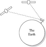
FIGURE 6.30 Global positioning system
A GPS receiver on the ground will attempt to receive time signals from as many satellites as possible and use the differences in those times, due to the time for the signals to travel, to calculate the position of the receiver.
GPS modules are generally a single IC, but require a special antenna that is usually the largest part of the module. Figure 6.31 shows the Venus 638 FLPx GPS module from SparkFun with its antenna attached. This module and modules like it have a serial interface that transmits a stream of updates giving the position of the receiver and various other information, such as the time and number of satellites currently being received.
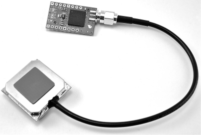
FIGURE 6.31 The SparkFun Venus638FLPx GPS module
..................Content has been hidden....................
You can't read the all page of ebook, please click here login for view all page.