5 DOMAIN-BASED TESTING

Everybody knows that there can be different goals for testing. For example, if the goal is finding defects in a software system, then a successful test is a test that makes the system perform incorrectly, hence exposing a defect. However, when the goal is to show that the software meets its requirements, then a successful test shows that the system operates as intended. In both cases, we need appropriate test data. Unfortunately, the entire input domain (the set of all inputs) is often infinite or extremely large, and we can conclude with the well-known fact that exhaustive testing is impossible.

Domain-based testing is a functional testing technique, in which the test design aims to reduce the number of test cases into a possibly small finite set, preserving the error detection or correctness retention capabilities. In domain testing, we view the program as a set of functions and test it by feeding it with some inputs and evaluating its outputs.

There are three techniques discussed in this chapter. The first is equivalence partitioning (EP). Here the input domain is divided into equivalence partitions, that is, into disjoint, non-empty, finite subsets. The test cases then cover each partition and verify the expected and unexpected computations.

Boundary value analysis (BVA) is another functional test technique in which the test case design concentrates on the boundary values between equivalence partitions. This technique checks if there are any faults at the boundaries of the domains.

The third technique, domain analysis, is an analytical way of computing the boundaries in those cases when the boundaries are functions of the input variables.

You may notice that these techniques are three aspects of the same domain investigation. That is why we group them and in practice use them together. You cannot select borders without knowing the equivalence partitions, which can be obtained by domain analysis.

EQUIVALENCE PARTITIONING

In domain testing, the first step is to partition a domain D into subdomains (equivalence classes) and then design tests with values from the subdomains. The equivalence classes (or partitions) are non-empty and disjoint, and the union of the partitions covers the entire domain D.

Test designers produce equivalence classes based on the specification. The equivalence classes are constructed in a way that inputs a and b belong to the same equivalence class if and only if the code for inputs a and b test the same computation (behaviour) of the test object (which states that the program handles the test values from one class in the same way).

Sometimes, during equivalence partitioning, the borders are determined from the code, where the variables in the predicates are computed from input variables. At this point domain analysis can be applied. However, the analysis here happens on the actual code, which turns the specification-based technique into a structured one. Hence, the technique can be applied in the test generation phase as well.

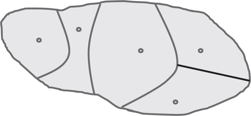
When the EPs are determined, it is mainly enough to select one input data from each equivalence class (see Figure 5.1).

In practice, we always start with determining first the valid, then the invalid partitions. This is especially important for BVA (see the section on boundary value analysis later in this chapter). Sometimes the given domain can be partitioned in different ways.

Fault models in EP

Selecting the test data from the partitions follows the rule: ‘A best representative of an equivalence class is a value that is at least as likely as any other value in the class to expose an error’ (Kaner, 2003). In practice, the input domain is in many cases multidimensional. In these cases, the test data selection depends strongly on the risk and the chosen fault strategy. In equivalence partitioning, we have two basic strategies: single vs multiple fault assumption.

Figure 5.1 Equivalence partitioning and test data selection

Example for EP – multiple fault assumption

Let’s assume that we have two (independent) input variables X and Y. Assume further that variable X has three EPs, X1, X2 and X3, while variable Y has four EPs, Y1, Y2, Y3 and Y4. We can test the system with four test cases, selecting a single pair of values from each EP, for example:

T1 = [x1, y1], T2 = [x2, y2], T3 = [x3, y3], T4 = [x1, y4].

Observe that one test case includes data from two EPs. If some test fails, we have to create additional tests to decide whether x_i or y_j is faulty. In some cases, we can solve the problem by applying special (e.g. null) values. For example, if X is a weight and Y is a size, both influencing the price of the delivery, then zero is a special value. In this case, we can create seven test cases.

Example for EP – single fault assumption

We have two (independent) inputs X and Y, where X has three EPs, X1, X2 and X3, while Y has four EPs, Y1, Y2, Y3 and Y4. We can test the system with seven test cases, selecting a single x_i or y_j value considering the EPs separately:

T1 = [x1, null], T2 = [x2, null], T3 = [x3, null],

T4 = [null, y1], T5 = [null, y2], T6 = [null, y3], T7 = [null, y4].

The single fault assumption is better for selecting concrete fault types and is more maintainable. The multiple fault assumption may result in fewer test cases. The right choice depends on the risks, which determine the chosen fault model.

Partitions exist in many areas of our software. It is the test designer’s task to safely and significantly reduce the testing effort by identifying and testing these partitions.

An example – authorisation

Authorisation version 1

Specification: A valid password must contain at least 8 and at most 14 American Standard Code for Information Interchange (ASCII) characters. Among the characters there has to be at least one lower case letter (a–z), at least one upper case letter (A–Z), at least one numeric character and at least one of the following special characters: ‘:’, ‘;’, ‘<’, ‘=’, ‘>’, ‘?’ and ‘@’. In the case of less than 8 characters the error message ‘The number of characters is less than 8’ appears. In the case of more than 14 characters, the error message ‘The number of characters is more than 14’ appears. In the case of a missing character type, the error message ‘Missing character type’ appears, showing one of the four types (lower, upper, numerical, special).

For this example, it is reasonable to focus on a single fault model.

Equivalence partition 1

The first test is always the happy path test, for which the password is correct. According to the specification, a password is correct if and only if:

The valid equivalence partition contains the passwords with properties above.

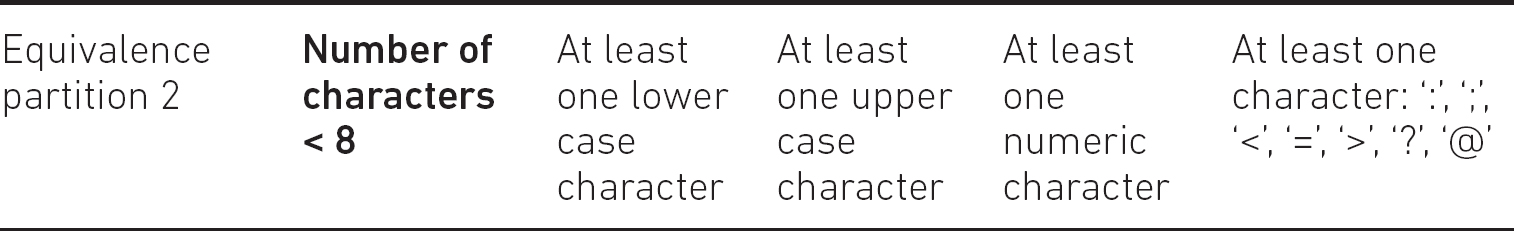
Equivalence partition 2

What are the other (invalid) equivalence partitions? Obviously, another partition can be when the number of characters in the password is less than eight, like ‘babE1=’. This can be our second equivalence partition. Also, this partition contains all the necessary characters, that is, upper and lower case character(s), number(s) and a special character(s) as well. This is because this partition then tests exclusively the passwords which are too short. A partition, which contains passwords having both too short and non-numeric characters, were inappropriate for the chosen model.

The test case selected from this invalid partition works in a way that for a short password, the result should be an error message ‘The number of characters is less than 8’. If the code were wrong, then instead of this message, the password would have been accepted (or an incorrect error message would appear).

Equivalence partition 3

The third – invalid – partition can be when the number of characters is greater than 14, such as ‘asdf1234ABC<?>@’. Also, similar to the first partition, this partition should contain all the necessary characters, that is upper and lower case characters, numbers and special characters as well.

Now, consider the next invalid partition. Starting from the error message ‘Missing character type’, we construct an equivalence partition where at least one of the character types is missing, while the number of characters is between 8 and 14. However, this partition is not appropriate. We have to separate the cases where lower case characters, upper case characters, numbers or special characters are missing. Therefore, we must have exactly four more equivalence partitions.

Equivalence partition 4

It contains upper case characters, lower case characters and numeric characters, but not any special characters from ‘:’, ‘;’, ‘<’, ‘=’, ‘>’, ‘?’, ‘@’. Also, the number of all the characters is between 8 and 14. An example is ‘Qwerty43’.

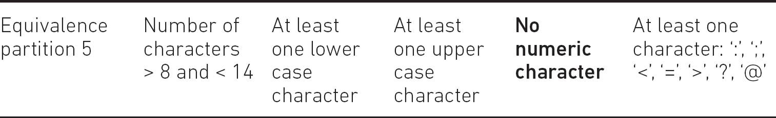
Equivalence partition 5

It contains upper case characters, lower case characters, special characters from ‘:’, ‘;’, ‘<’, ‘=’, ‘>’, ‘?’, ‘@’, but not any numeric characters. Also, the number of all the characters is between 8 and 14. An example is ‘Man>=Boy’.

Equivalence partition 6

It contains upper case characters, numeric characters, special characters from ‘:’, ‘;’, ‘<’, ‘=’, ‘>’, ‘?’, ‘@’, but not any lower case letters. Also, the number of all the characters is between 8 and 14. An example is ‘WOMAN=42’.

Equivalence partition 7

It contains lower case characters, numeric characters, special characters from ‘:’, ‘;’, ‘<’, ‘=’, ‘>’, ‘?’, ‘@’, but not any upper case letters. Also, the number of all the characters is between 8 and 14. An example is ‘rose11;;’.

Equivalence partition #8

A partition for inputs outside all of the partitions above.

Clearly, the first seven equivalence partitions do not result in full partitioning. It is easy to see that there are other partitions in the domain space, but these contain data violating our fault model. Such an example is ‘aaaa2222’, which is not in any EPs of those listed (it is not on the happy path, it contains neither an upper case character nor a special character). Hence, the tester either gives up the single fault model or does not choose test data from the remaining invalid partition(s). In the first case there are 11 other partitions to consider (with sample data ‘########’, ‘aaaabbbb’, ‘QWERTYUI’, ‘66666666’, ‘=<>??@:;’, ‘aaaa2222’, ‘LADYemma’, ‘dady@com’, ‘PAWN1234’, ’BOY?GIRL’, ’::;;9876’). In the second case, insisting on the fault model, we do not choose data from the 8^th partition.

Insisting on the single fault model, Table 5.1 shows the equivalence partitions.

Table 5.1 Equivalence partitioning for the authorisation example

In Table 5.1, bold represents the error-revealing partitions assuming the single fault model. If a test fails, then the bug relates to exactly one of the partitions.

Finally, based on the equivalence partitions we design the test cases. We simply select one test from the first seven partitions. A possible solution can be the following (test cases for EPs in the authorisation example):

The authorisation example also shows that the fault model determines the partitions, and hence, the number of tests.

BOUNDARY VALUE ANALYSIS

Equivalence partitioning is rarely used in isolation. Potential bugs occur ‘near to the border’ of the partitions with higher probability. As Boris Beizer said, ‘Bugs lurk in corners and congregate at boundaries’ (Beizer, 1990). The reason is that the implemented and the correct borders are often different. The question is how to select the test cases concerning the boundaries. Note that different textbooks suggest different solutions. We show in this section why the test selection criterion presented here is worth applying.

Before we continue, let’s define some important notions:

The ON and OFF points have to be ‘as close as possible’. This means that if an EP contains only integers, then the distance of the two points is one; for example, if an EP contains book prices, where the minimum price difference is EUR 0.01, then the distance between the points is also EUR 0.01.

For example, in the TVM specification, the minimum price shift is EUR 0.1.

Fault models in BVA

There are two types of fault models in BVA: predicate faults and data (variable, operator) faults.

Predicate faults

Assume that a valid equivalence partition contains integer values greater than 42. A correct implementation of this partition can be:

if Age > 42 then …

The potential error can be any other implementation of the predicate. Table 5.2 shows the error detection capabilities of BVA for various predicates (shaded boxes mean that an error has been detected for a given test case).

Table 5.2 Test design against predicate faults. BVA for predicate Age > 42

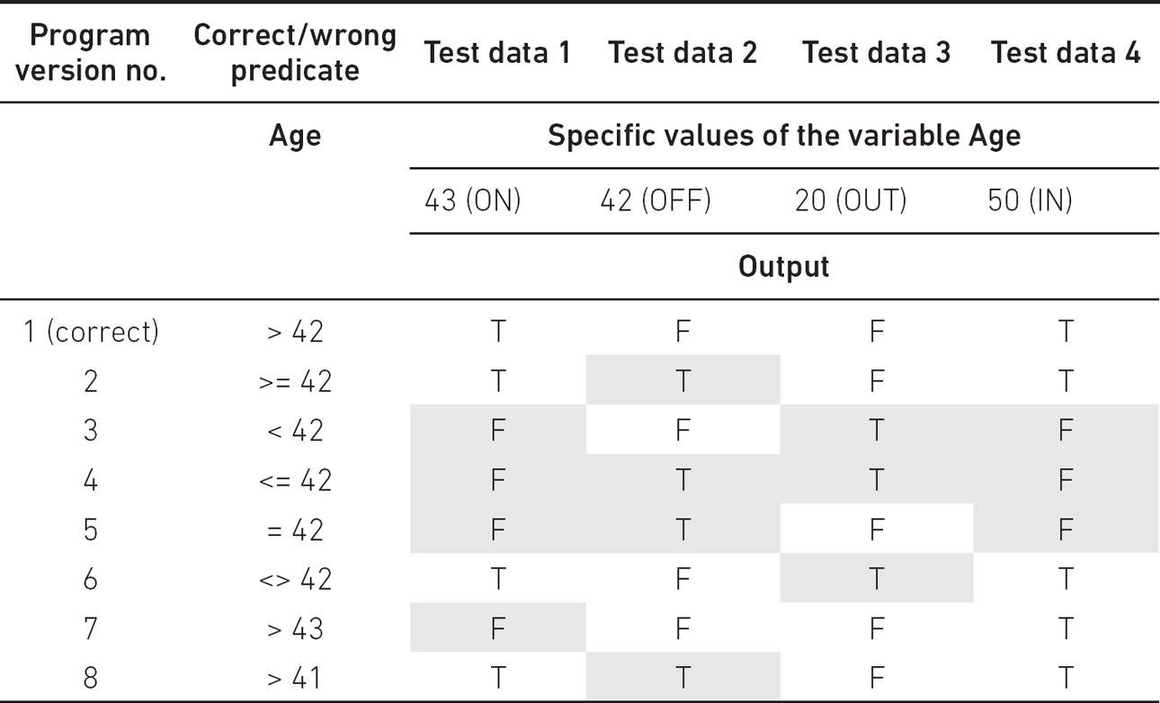
We can see that the first three test data are necessary to detect all possible errors, while the fourth one is superfluous. We can also see that for program version 7, test data 1 will detect the bug for > 44, > 45 and so on. Similarly, for program version 8, test data 2 reveals the bug for > 40, > 39 and so on. Therefore, the BVA requires three test cases (see Figure 5.2).

Figure 5.2 Equivalence partitioning with ON/OFF/OUT points for open boundary

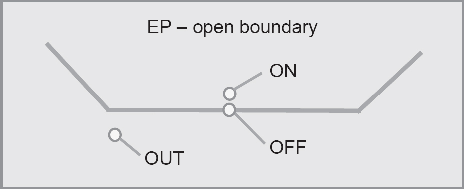
In practice, we have to test the neighbour partitions as well. The OUT point can be any ‘middle’ point outside the boundary. The ON point of the neighbour is just the OFF point of our original partition, therefore one ON and one OFF point is enough. But what about the ‘extreme’ partitions, where no neighbour partitions are serving ON points in this way? In this case, we have to consider the ‘limit’ values, bounded by some (specification or computer hardware) constraint. For example, if the valid partition is bounded by x < 5, where x is an integer, then the limit value is the smallest negative integer representable by the programming language or hardware architecture. Obviously, it can be implementation or architecture dependent, which has to be considered in the implementation phase.

Let’s consider the case when the correct implementation is a ‘greater than or equal to’ border:

if Age >= 43 then …

Table 5.3 demonstrates this point.

In this case, also three test cases are required (for test data 1, 2 and 4, see Figure 5.3). However, they are different from the ones previously seen.

Table 5.3 Test design against predicate faults. BVA for predicate Age >= 43

Figure 5.3 Equivalence partitioning with ON/OFF/IN points for closed boundary

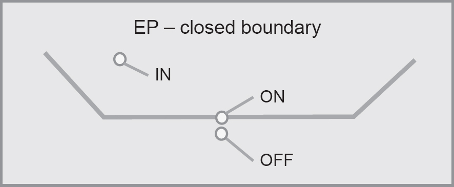
Similar to the previous case, one ON and one OFF point are enough, since an IN point is an OFF point of a neighbour partition.

Now let’s consider the following predicate:

if Age == 43 then …

This is demonstrated by Table 5.4.

Table 5.4 Test design against predicate faults. BVA for predicate Age == 43

In this case, three test cases are required as well. All of the following triples are reliable (test data 1, 2 and 3), (test data 1, 2 and 5), (test data 1, 3 and 4), (test data 1, 4 and 5). This means that one ON and two OFF/OUT points are reliable when the two OFF/OUT points are on the opposite side of the border (see Figure 5.4).

Figure 5.4 Equivalence partitioning with ON/OFF/OUT points for closed boundary from both sides

For simplicity, we can use the same solution as above, that is requiring an ON–OFF pair and a third point, which can be an ON point of another border (or limit value) on the other side of the OFF point.

Finally, for the predicate

if Age <> 43 then …

the reliable solution is as per Figure 5.5.

Figure 5.5 Equivalence partitioning with ON/OFF/IN points for open boundary from both sides

Observe that one ON–OFF pair and one IN/OUT point is reliable for all the examined predicate faults above. The IN/OUT point can be the OFF/ON point of the neighbour partition.

Data faults

Let’s consider the following data fault, where badVariable is used instead of Age:

if badVariable >= 43 then …

If Age is incorrectly changed to badVariable, then an ON–OFF pair is reliable for revealing the fault (see Table 5.5).

The only additional requirement is that we have to keep all the other variables (except Age) unmodified. You can see that the ON point reveals the defect of badVariable being 42 and 20 (diagonal), while the OFF point reveals the other incorrect values of badVariable (darker grey).

Now let’s consider the fault:

if badVariable == 43 then …

Again, an ON–OFF pair is enough to detect the bug, and it is true for all other cases when only one variable is wrong in a predicate (see Table 5.6).

Table 5.5 Test design against data faults. BVA for badVariable >= 43

Table 5.6 Test design against data faults. BVA for badVariable == 43

Similar is the case for predicates with more variables. Consider this correct predicate:

if Age + otherVariable >= 43 then …

One variable mistake can happen as a result of a change, for example replacing otherVariable with wrongVariable. This case is similar to the one above. Another variable error is omitting otherVariable. To test this case reliably, we should avoid degenerate values of variables, here otherVariable = 0. Therefore, set all the variable values to non-zero, non-empty string and so on.

Finally, let’s consider the case when the correct predicate is:

if Age >= 0.5 then …

Let the accuracy of the data type of the variable be 0.01. If the incorrect implementation is

if 1.01 x Age >= 0.5 then …

then Table 5.7 applies.

Table 5.7 Test design against data faults. BVA for bad constant

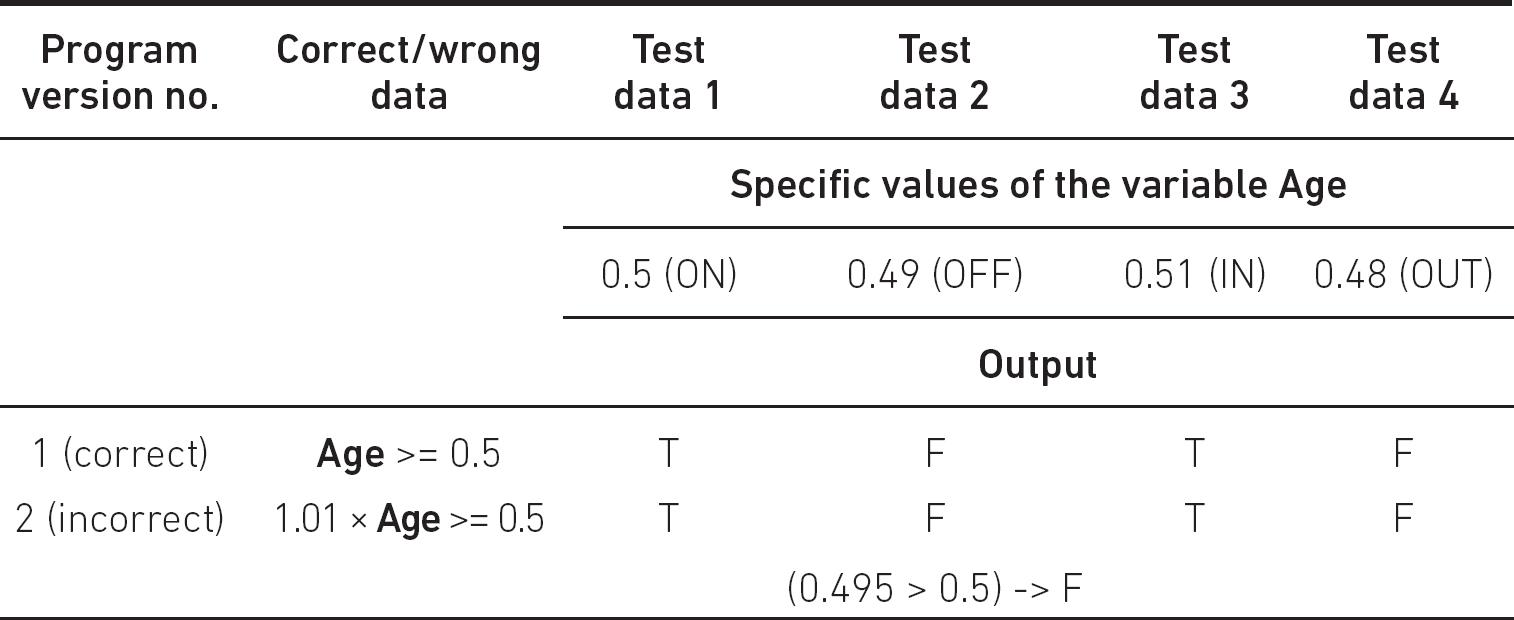
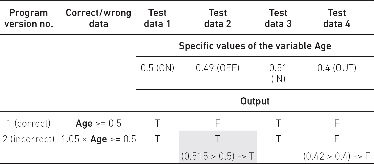
No test case reveals this ‘bug’. However, this is not a real bug as for each value of Age the same branches will be executed; therefore here the two implementations are ‘identical’. When the incorrect implementation is

if 1.05 x Age >= 0.5 then …

then our tests become reliable (Table 5.8).

Here the OFF point reveals the bug, that is the ON–OFF pair is error revealing in this case as well (or the jumps to branches are identical).

Testing a boundary requires setting other input data, which is not related to that boundary. If we follow the single fault assumption, we will set these variables as IN points of the related domains.

Table 5.8 Test design against data faults. BVA for other bad predicate

EP and BVA together

Equivalence partition testing and boundary value analysis are used together. The former is weak without the latter, while boundary value analysis can only be used if we know the equivalence partitions. When designing the test cases, we explore equivalence partitions first, and then, knowing the boundaries, we design the tests to fulfil both methods together.

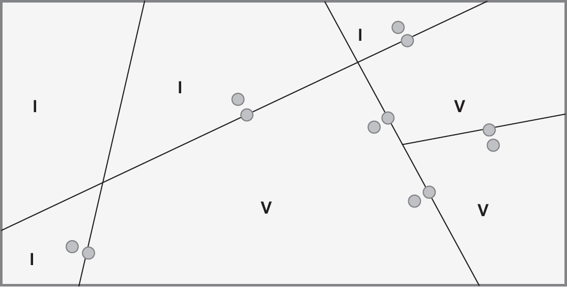
We mentioned earlier that differentiating valid and invalid partitions is very important for boundary value analysis. The reason is that it is superfluous to test a boundary between two invalid partitions. Consider Figure 5.6 where we separate the valid and invalid partitions.

In Figure 5.6 ‘I’ denotes invalid and ‘V’ denotes valid partitions. We can see that we test the borders between (valid, valid) and (valid, invalid) partitions. However, we never test a border between (invalid, invalid) partitions.

Since test cases on or near to the boundary may reveal more defects than test cases of inner points, ON points may detect multiple defects, that is both computation and domain errors.

We have seen that for BVA an ON–OFF pair is enough since the necessary IN/OUT points are usually covered by other partitions. However, when we need an ON, OFF, OUT triple, we have no IN point. The question is whether in this case the ON point is enough or not. In the case of a single ON point we do not always know whether it is a computation error (erroneous computation resulting in an incorrect result) or a predicate error (due to an erroneous condition). Selecting a single ON point, our testing satisfies the multiple fault assumption. However, in many cases, we still know which of the error types occurred. In the case of a predicate/domain error, the control (execution) goes along another input domain, and we know the expected result of the neighbour domain. Therefore, except for some coincidences, it is superfluous to design two test cases, that is one ON and one IN point.

Figure 5.6 Valid and invalid partitions with ON-boundary points

Example

In this case, testing with input x1 = 10 (ON) and x2 = 9.9 (OFF), the results are a = 100 and 98.01. Therefore, the ON point shows a predicate error since 12 is expected, which is computed in a different branch. The OFF point (a = 98.01) shows a computation error since 19.8 is expected.

This knowledge permits us to design minimal but still reliable tests. Other test selection criteria found in textbooks or blogs may result in significantly more test cases. Let’s consider the most frequent case when we have linearly ordered partitions (see Figure 5.7).

In this case, our test selection criterion requires 4 ON, 4 OFF and one IN/OUT points. If we have N domains in this simple arrangement, then the number of test cases is 2N – 1, which can be extended by special test cases containing special values.

Summarising, we have a test selection criterion for the combined EP and BVA method that is identical with the test selection criterion for BVA.

Figure 5.7 Linearly ordered partitions

Example for BVA (continued from EP)

Now let’s consider the equivalence partitions in our previous example. For clarity, we start with the test cases other than the happy path:

The ON-boundary value here is 7, the OFF-boundary is 8 and the OUT point is 14. The OFF-boundary and the OUT point will be the boundary of the happy path. Here, we consider only one input characteristic, that is the length, while the others remain unchanged. Since we intend to test whether the length of the password is not too short, all other characteristics are irrelevant. That is, we can select any characters that meet the related characteristic, for example ‘aa’ + ‘BB’ + ‘33’ + ‘:’. These strings fulfil the above characteristics, respectively. Considering EP3:

The ON-boundary is 15, while the OFF-boundary is 14, and the OUT point is 8, which are also located on the boundary of the happy path. Let’s go on:

At first sight, all the special characters seem to be equivalent. However, a professional developer does not consider these characters one by one. Instead, they know the ASCII code of these characters, which makes it possible to handle all these characters together. Here, ‘:’ has the smallest, while ‘@’ has the highest, ASCII code, that is 58 and 64, respectively, which are the OFF-boundary characters of EP4. These OFF-boundary values are just ‘:’ and ‘@’, which are also the boundary of the happy path.

These points can also be considered as OUT points. When ‘:’ is the OFF point, then ‘@’ is the OUT point and vice versa. Here we would just like to demonstrate our assertions that an ON–OFF pair is enough; the OUT/IN points are ON/OFF points of the neighbour partitions. From here we only consider the ON–OFF pairs.

The boundaries are 57 and 65, which are the closest non-special characters. These are just the ASCII codes of 9 and A, respectively.

In EP5 the OFF-boundary values are 0 and 9, which are the boundary values of the happy path. The boundary values, that is the closest non-numeric characters, are ‘/’ and ‘:’, respectively. The second is a boundary value of the happy path.

In EP6 the OFF-boundary values are A and Z, respectively, which are the boundary values of the happy path. The boundary values, that is the closest non-upper case characters, are ‘@’ and ‘[’, respectively. The first is a boundary value of the happy path.

In EP7 the OFF-boundary values are ‘a’ and ‘z’, respectively, which are the boundary values of the happy path. The boundary values, that is the closest non-lower case characters are ‘`’ and ‘{’, respectively.

Since the OFF-boundary values of the non-happy path test cases are just the boundary values of the happy path, considering equivalence partitions 2–7 gives all the necessary boundaries.

Based on these ON-boundary and OFF-boundary values the complete test set can be constructed. We aim to minimise the number of the test cases. Unfortunately, we have to do this optimisation manually. Note that the different sub-boundaries are independent, hence, we can set more ON-boundaries in one test case.

Table 5.9 contains the test design of the above example. Here, the table contains the type and the ID of the test cases with their descriptions, and the OFF-boundary pairs of the (boundary) test. Here ‘V’ means valid, ‘I’ means invalid, ‘C’ relates to the partition (class) and ‘B’ relates to the boundary, for example ‘VB’ is a valid boundary test (ON point).

Table 5.10 contains the test case IDs, the input, the expected output and some comments. Here we only consider boundary test cases. It is cost-effective since if a test, whose probability is low, fails, we can add a ‘mid-boundary’ test case to help the developer to know whether the bug is due to a faulty border or a computation defect.

Table 5.9 Test design for the ‘Authorisation’ example

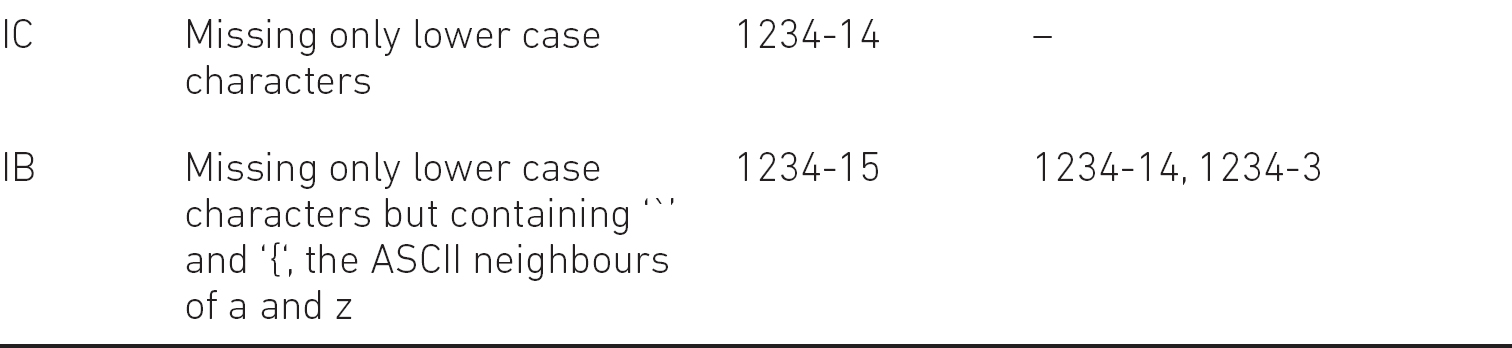
Table 5.10 Test cases for the ‘Authorisation’ example

We can see that the number of test cases is increased only by one. This is because 1234-2 involves many independent boundaries and since passwords contain multiple characters, we can cover more boundary characteristics in one test case. One exception is the length of the happy path, which cannot be 8 and 14 at the same time.

Example: Authorisation Version 2

Specification: A valid password must contain at least 8 and at most 14 ASCII characters. Among the characters there has to be at least one lower (a–z), at least one upper case letters (A–Z), at least one numeric and at least one of the following special characters: ‘:’, ‘;’, ‘<’, ‘=’, ‘>’, ‘?’ and ‘@’. In the case of less than 8 characters, the error message ‘The number of characters is less than 8’ appears. In the case of more than 14 characters the error message ‘The number of characters is more than 14’ appears. In the case of a missing character type, the error message ‘Missing character type’ appears showing one of the four types (lower, upper, numerical, special).

Version 2 is very similar to the original, therefore even taking into account the competent programmer hypothesis, a developer may implement it incorrectly. This specification has to be tested by a slightly different test case set. Namely, test case T1234-11 = {/cdHU:tGaaV} would be superfluous for Version 2, since it would test the same equivalence partition (the happy path) as T1234-2. Therefore, we justified the necessity of T1234-11 by this alternative specification.

On the other hand, if T1234-11 were missing, then Version 2 would reveal it.

Similarly, you can easily imagine alternative specifications for all test cases from T1234-5 to T1234-13, while the tests for a happy path are obvious.

This example shows the essentials of black-box mutation testing, which is a method for validating whether our test cases are well designed without executing the test cases. If you are not sure whether a given test case is necessary or not, just imagine a slightly modified specification, which makes this test necessary in the original, and superfluous in an alternative one. If you could not find it, maybe it is superfluous. If you could imagine a slightly alternative specification for which you believe that the EPs, the boundaries and thus the test cases are just the same, then you have probably missed some tests.

It is not necessary to construct all the EPs and boundaries; just consider the modified part and the EPs related to this modification, for example modifying the specification part from

to

you have to investigate only EP5 and EP6.

The specification has to contain the EP to be validated in such a way that only a test case from this EP would detect the defect. If the alternative specification is far from the original, then it can be ignored. If the specification is close to the original, the EP has to be considered. Fortunately, black-box mutation analysis can be used for both cases.

DOMAIN ANALYSIS

We have considered so far the cases when EPs can be generated based on one input variable directly. In practice, however, predicates are functions of more variables, such as 2x + 5y + k, where k = z/4 +1, and x, y, z are input variables. White and Cohen (1980), who introduce domain testing, investigated the types of predicates. Their result is language independent since the predicates reflect the specification. They found that more than 10 per cent of the predicates contain more than one variable.

In the case of more complex predicates, the domains are determined by domain analysis. In the simplest cases, the domain analysis is straightforward and can be done at the test design phase. In complex cases, the task may be unsolvable.

Example: taxi driver’s decision – go/no go

The taxi driver knows the following:

We assume that the driver wants to earn at least EUR 20 for each ride, the precision of measuring d is 0.1 km, the time accuracy is 0.1 hour. Then, the fare of a ride is 2 + 16 x t-ride (hour) + d (km). The driver cannot accept a reservation that would exceed t-full = 10. The starting time is calculated by the engine, and should be between zero and t-full. The program computes whether the driver should go or wait for another call.

For example, if the ride takes 45 minutes and the distance is 5 km (huge traffic jam), then they earn 2 + 12 + 5 = 19 EUR, which is below the limit, and thus, they reject this passenger.

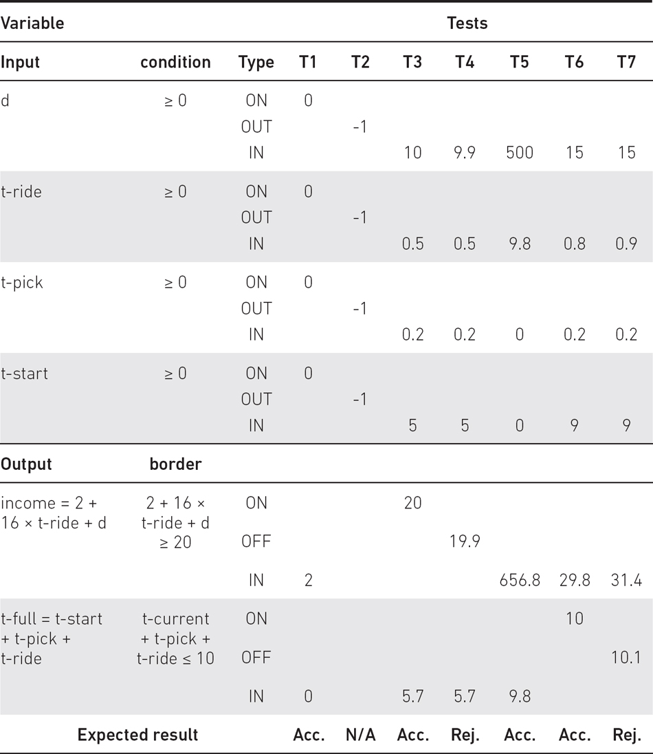
The input variables d, t-start, t-pick and t-ride have to be non-negative. These conditions seem to be borders. However, at the current state-of-the-art of development, input handling is addressed by applying existing frameworks. It means that when we apply the chosen framework correctly, we do not have to test the predicate d >= 0 (since it is the framework). As a consequence, this condition has to be tested only with two values: (1) d = 0; (2) d < 0. Value (2) is necessary because the developer may set the framework incorrectly, so that negative values may occur.

Test for (1) is just an ON point, and test for (2) is an OUT point, but here OUT means ‘outside the input domain’. To test this OUT point, checking the existence of the sign ‘–‘ may be enough. No IN point is required when testing these conditions. With one ON and one OUT point, we are able to test the integration of our application with the framework. All these necessary tests can be done by two test cases: T2 involves the testing of non-enabled negative values, while T1 involves zero for all inputs (see Table 5.11). This is a real case, for example when somebody stops a taxi but changes their mind.

The border with regards to the necessary income is:

2 + 16 x t-ride + d >= 20.

The border with regards to the time limit is:

t-start + t-pick + t-ride <= 10.

Considering the first border, the ON point (T3 in Table 5.11) can be determined by solving this equation:

16 x t-ride + d = 18.

A realistic and simple solution is when t-ride is 0.5 (30 minutes) and

d = 18 – 16 x 0.5 = 10.

The OFF point (T4) is when we reduce either the distance by 0.1 km or the time by 0.1 hour. Considering these cases we obtain:

OFF1: 2 + 16 x 0.4 + 10 = 18.4

OFF2: 2 + 16 x 0.5 + 9.9 = 19.9

where the latter is a valid OFF point. According to our test selection criterion we need an IN point (T5), since our partition, 16 x t-ride + d >= 18, is an edge partition. Let’s select a very large IN point: t-ride = 9.8, and d = 500; since t=ride < 10, t-start = 0, t-pick = 0. The result is 656.8.

We determine the values of the other variables later. Now consider the other border.

t-start + t-pick + t-ride <= 10.

For a realistic solution let the pickup time t-pick be 0.2 and the paid time t-ride be 0.8 and d =15. With this, t-start = 9 resulting in an ON point (T6): (9 + 0.2 + 0.8 = 10). The OFF point (T7) has to be 10.1 and we can increase t-ride to 0.9.

We have to test the IN point as well; however, this has been tested by T5.

The variables, which are outside a predicate, are used satisfying the single fault assumption. For example, in the case of testing the OFF2 point, t-start and t-pick is selected in a way that t-start + t-pick + t-ride << 10.

A domain test matrix is used to make the choice of the boundary values more convenient and easier. Here the necessary information is represented in the form of a table. This helpful technique was suggested by Binder (2000).

You can see that in selecting ON/OFF points for a given border we always select IN points for the other border to satisfy single fault assumption.

Table 5.11 Test design for the ‘Taxi driver’ example

Extending this example, we easily get non-linear borders. We can assume that the driver wants to earn EUR 20 in one hour instead of gaining EUR 20 for a ride. In this case, the border is non-linear – the interested reader can easily determine the predicate for this case. According to our knowledge, there is no accepted theoretical result for this rare case; we suggest applying more ON/OFF/IN data.

CHALLENGES IN DOMAIN-BASED TESTING

The fault assumption for domain-based testing is that the computation is correct, but the domain definition is wrong. An incorrectly implemented domain means that the boundaries are wrong, which may induce incorrect control flow. In this section we summarise the possible domain problems.

Possible domain problems:

As you can see, the partitioning questions raise the problems of deeper boundary analysis. That is why we have to discuss it in more detail.

TVM EXAMPLE

Let’s select specification ‘Buying process’ from our TVM example. For this chapter, extending it with the acceptable banknotes:

Note that in the previous chapter we extended the specification so that the admin of the ticket machine company will be able to modify the ticket prices. Therefore, we assume that the ticket prices can be set to any amount. We also consider the granularity of the ticket price of 0.1 EUR.

Let’s consider the text in italics first. The examples in this specification help us in selecting the equivalence partitions. We have two inputs: (1) the remaining ticket price and (2) the set of available banknotes. It is very important that the set of acceptable banknotes is constant and not a variable. Therefore, though we have to consider it when constructing the EPs, we can create the partitions without involving this set, since every partition will contain the same elements. Let’s start with the partitions of the ticket prices.

Let the remaining amount to be paid (RAP) be:

Considering the acceptable banknotes, we can construct Table 5.12. We assume here that the remaining amount to be paid is always positive.

Table 5.12 Acceptable banknotes for TVM

EP	RAP in EUR	Acceptable banknotes
1	<= 5	€5
2	> 5 and <= 10	€5, €10
3	> 10 and <= 20	€5, €10, €20
4	> 20 and <= 50	€5, €10, €20, €50
5	> 50	€5, €10, €20, €50

We can easily observe that EP5 can be merged with EP4 since the acceptable banknotes are the same. The table has been updated as Table 5.13.

Table 5.13 Acceptable banknotes for TVM – improved

EP	RAP in EUR	Acceptable banknotes
1	<=5	€5
2	> 5 and <=10	€5, €10
3	> 10 and <=20	€5, €10, €20
4	> 20	€5, €10, €20, €50

Instead of selecting one test case from each partition, we move forward to include boundary value analysis. According to Table 5.13 we have four EPs and according to our test selection criterion we design three test cases for each EP – we restrict them to the input values only:

We selected the first IN point as the minimum possible amount. Considering EP2 and EP3, they have two ON/OFF points and one IN/OUT point because of the two borders. Because of the same values in different EPs, we have 7 test cases instead of 14. To make our tests complete, we extend the test cases with the ticket price and the inserted amount of money; see Table 5.14 for the designed test cases.

Table 5.14 Test cases for TVM

Note that here we only test the software of the machine and we cannot test the ‘hardware’ by inserting non-acceptable banknotes. Of course, the hardware has to be tested by inserting non-acceptable banknotes and other banknotes, for example smaller value foreign banknotes such as HUF 500 (< 2 EUR).

What we can learn from this example is the following:

Summarising, applying EP and BVA is not an easy task but is challenging and interesting for testers.

Finally, let’s consider inserting coins: payment is possible by inserting coins or banknotes. There is not too much information on inserting coins. Since there is not any restriction, we can select a unique happy path where the input is a set of all the acceptable coins and where each coin type is inserted more than once. Another possibility is that coins are tested for another specification (user story), where coin insertion is more relevant.

METHOD EVALUATION

Domain-based testing is perhaps the most widely used test design technique. This is because it is easy to use and lots of real specifications require the application of it. In this section we summarise its applicability, advantages and limitations.

Applicability

These techniques are applicable at any levels of testing. Moreover, the presented domain testing methods can rarely be used in isolation, and are applicable mainly in stateless cases. Roughly speaking, we can apply them if all the inputs are available at the initial state, and no input can be entered into a special state.

However, we show that different test design methods can be used together for some specifications. If the program is in a given state, we can apply EP and BVA as in the case of a stateless code.

Types of defects

The methods are especially useful for domain errors, that is when predicates in the conditional statements are faulty. The methods are also beneficial for detecting simple computational errors, which may occur along the execution paths inside the equivalence partition.

Advantages and shortcomings of the method

The advantages of EP, BVA and the domain analysis methods are the following:

The limitations and shortcomings of EP, BVA and the domain analysis methods are the following:

THEORETICAL BACKGROUND

The theory of domain-based testing dates back to the 1970s, when testing research started. Unfortunately, testing theory in general is rarely used in practice, but domain-based testing is a refreshing exception.

Partition Testing

Partition testing is one of the oldest testing methods, first mentioned in a paper by Goodenough and Gerhart (1975). EP is a special case of partition testing where the partitions are disjoint. In EP testing, we call a domain partitioning homogeneous if either all of its members cause the program to pass or all cause it to fail. Weyuker and Ostrand (1980) used the term ‘revealing’ for homogeneous partitions. A very good description about partition testing comes from Hamlet and Taylor (1990). They state that ‘specification-based subdomains are particularly good at detecting missing logic faults, which are the most common programmer mistakes’.

In general, partitions are not necessarily disjoint; they may overlap. In this case, we cannot call them partitions, but rather overlapping subdomains. This is the case for statement testing, which is a white-box testing strategy, where the program statements have to be covered. Here the subdomain relation is the following: two inputs are in the same subdomain if they cause the same set of statements to be executed. Since one input may cover many (different) statements, the subdomains are overlapping. The case for mutation testing is similar.

The reliability of equivalence partitioning was investigated in different case studies. Reid (1997) investigated EP, BVA and random testing for real code with real bugs. He found that BVA was much more reliable than EP. However, the number of test cases were three times more in BVA than that of EP. We considered these methods together and suggest not using EP in isolation.

In Arnicane (2009) the author described several test selection criteria for EP and BVA. She referred to the original single fault solution as weak equivalence class testing. She considered the combinatorial extension of EP as strong equivalence class testing. The paper differentiates between inner and outer OFF points, where inner OFF points are actually ON points close to the border. With this, the author introduced weak IN and OFF boundary testing, where each (ON–inner OFF), (ON–outer OFF) pair is tested, extended by an inner value of the EP. When both IN and OFF boundaries are tested with an inner test case, she calls it ‘robust weak boundary value testing’. It is not clear which out of the test selection criteria have to be applied in which situation. This author prefers single fault solution with one ON–OFF pair of test cases.

Domain testing in general

One of the basic errors in software is domain error (Howden, 1976), which occurs when a specific input follows a wrong path because of an error in the control flow of a program. This type of error can be revealed by applying a domain testing method introduced by White and Cohen in 1980. Since the faulty domain can be very close to the correct one, input data near the boundary of a domain partition are therefore more sensitive to program faults and should be carefully tested.

The idea of domain testing is to detect these types of faults by carefully selecting data that are on and near the boundary of the path domain. White and Cohen’s method requires two ON and one OFF points for a simple linear two-dimensional border. Jeng and Weyuker (1994) presented a simplified domain testing strategy where a linear border in any dimension is tested by one ON and one OFF point.

The design for domain testing can be supported by automatically generating the ON and OFF points. However, generally, it is very costly. A heuristic approach published by Jeng and Forgács (1999) addresses this difficulty.

We can see that domain testing may offer a white-box alternative to boundary value analysis. BVA intends to find particular domain errors. Domains have to be (implicitly or explicitly) described in the specifications. Since a significant portion of bugs are domain errors, we can now understand why this method is very successful (see Reid, 1997).

KEY TAKEAWAYS

Any software can be viewed as a function mapping from an input domain to the output domain. Domain-based testing focuses on the classification aspect of the input and explores incorrect boundaries and computations.

EXERCISES

E5.1 Identify the EPs and one ON, OFF and IN/OUT point for each EP in the following specification.

Payment: for online shopping, the shipment fee is the following. If the final price is below EUR 50, then the shipment is not possible. If the price is below EUR 100, then the shipment fee is 10 per cent of the final price, in the case where the price is below EUR 500 the shipment fee is five per cent, and if the price reaches or exceeds EUR 500, the shipment is free. If the weight surpasses 10 kg, then EUR 1 is paid for each kilogram (where weight is rounded up to the next integer). Finally, if the shipment comes from abroad, the extra fee is doubled except for neighbouring countries, where the extra fee is only 1.5 times more. The price shift is EUR 0.1; the minimum non-zero weight shift is 0.1 kg. No negative or non-numeric cases should be considered.

E5.2 Produce a test design for the specification above.