
6 STATE TRANSITION TESTING
WHY IS THIS CHAPTER WORTH READING?
State transition testing models the behaviour of an application or system for different input conditions. Behaviour here means the full expected functionality. In this chapter you will learn the difference between stateless and stateful applications, the main concepts of describing states and transitions and how to apply state transition testing (STT) in test design. You will learn how to use STT on its own, or together with EP and BVA. We introduce two test selection criteria: all-transition-state coverage and all-transition–transition coverage, which are relatively ‘cheap’ with high defect detection capability.
STATEFUL AND STATELESS SYSTEMS
In the previous chapter, we considered test techniques for stateless software. Statelessness means computational independency on any preceding events in a sequence of interactions. A stateless application decouples the computations from the states; it is dependent only on the input parameters that are supplied. Simple examples are:
• a search function in a text editor with a given search pattern;
• a sort function with given items to be sorted;
• a website that serves up a static web page (each request is executed independently without any knowledge of the previous requests) and so on.
In these cases, a stateless system/function returns the same value for the same arguments. The computations are replaceable without changing the behaviour of the application.
On the other hand, stateful applications have internal states. These internal states need some place for storage (allocated memory, database, etc.). When a stateful function is called several times, then it may behave differently. From the test design point of view, it is more difficult to test since it must be treated together with the preceding events. An operating system is stateful. If you set your screen resolution, next time you switch on your machine, this resolution is preserved.
STATES, TRANSITIONS, CONDITIONS
Most complex systems are stateful. Many of them are event-driven (or reactive) in which they wait continuously for some external or internal event (mouse click, time tick, data packet, button press, etc.), and after recognising the event, react to them by performing some computation or by triggering other software components. Such systems can have more than one state and exhibit different behaviours in different states. There can be various transitions between the states.
There are two main ways to represent stateful systems: using state transition diagrams (graphs) or state transition tables. In the first case, the nodes represent states and the edges represent transitions. If the system is in state s1, and an input event/trigger E occurs, then the system changes its state to s2 via the transition t, producing the output action O (see Figure 6.1).
Figure 6.1 State transition diagram. A transition t occurs from state s1 to s2, which is triggered by some input event E and resulting in an output action O

Roughly speaking, a transition consists of a start state + an input event + an action + a next state. In an extended model, the transition and the resulting state may also depend on some conditions. For example, by clicking on the ‘+’ button next to some food to be ordered, if the maximum number of the ordered item has been reached, then nothing happens, while in other cases the ordered amount is incremented. Such guard conditions are usually denoted by Event/[condition]/Action.
It is important to note that for any given state an event can cause an action (or set of actions), but the same event – from a different state – may cause a different action and transitions to a different state. In practice, an action set may include programming elements, that is code.
There are two common ways to arrange state transition data in a table.
1. All the states are listed on the left side, and the events are enumerated on the top. Each cell in the table represents the next state and the action list of the system after the event has occurred (see Table 6.1).
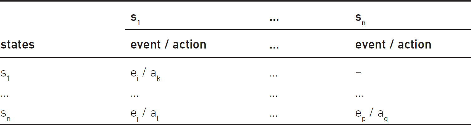
2. All the originating states are listed on the left side and the resulting states on the top. Each cell in the table represents the event/action list of the system (see Table 6.2).
Table 6.1 State–event notation for a state transition table
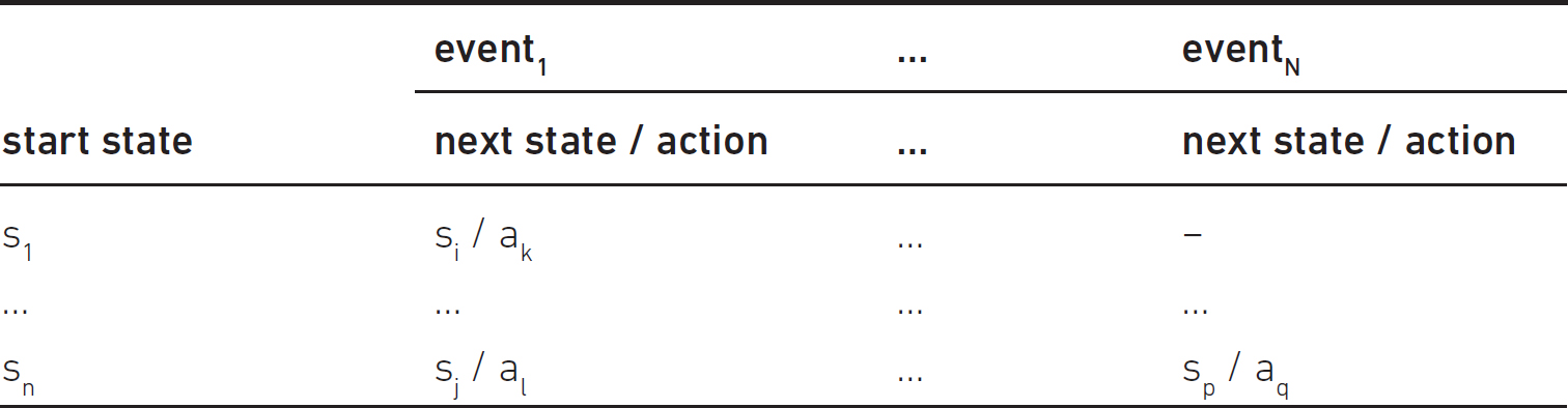
Table 6.2 State–state notation for a state transition table
Note that an action may consist of independent, simple actions. Valid transitions are transitions described in the model (see Figure 6.1 and Tables 6.1 and 6.2). However, there can be some undefined (‘−‘) transitions in both tables. These transitions may mean that the specification is incomplete; therefore the tester should analyse undefined transitions thoroughly.
In practice, incomplete specifications can be handled in two ways: (1) the system does not change its state, and there is no output (the undefined transition meets the specification) or (2) there should be a transition to an error state (each event should be handled). An invalid transition refers to the transition that transforms the system into a state that causes the incorrect or undefined behaviour of the system, indicating that such transitions are not feasible. In some cases, it is useful to use a transition without any output (e.g. allocating a resource that is not available, or a timeout happens). We call these null transitions. Null transitions can have guards (for example, [timer = 3]). Note that undefined or null transitions are not necessarily invalid.
A state transition graph always has a start and may have one or more end nodes. Each node has to be accessible from a start node, and loops in the graph are allowed.

Mathematically speaking, a state transition diagram (state diagram) for a finite-state machine (FSM, finite automaton) is a directed graph with (S, E, O, δ, q0, F), where S denotes the finite set of states, E denotes the finite set of input symbols (events), O denotes the finite collection of output symbols, δ : S x E → S x O (the transition function), q0 is the start state, and F denotes the set of final states (if used).
A Mealy Machine is an FSM whose output depends on the actual state as well as the actual input. A Moore machine is an FSM whose output depends on only the actual state. The finite automaton is deterministic (DFA) if each transition is uniquely determined by its source state and input symbol, and reading an input symbol is required for each state transition. Otherwise we call it non-deterministic. DFAs are used in formal language theory in describing regular languages. The deterministic and the non-deterministic automaton have the same ‘power’, that is they both recognise the same formal language.
State machine minimisation (reduction) identifies and combines all states that have equivalent behaviour. Two states have equivalent behaviour if, for all input combinations, their outputs are the same and they change to the same or equivalent next states. Hopcroft’s algorithm finds the minimal deterministic automaton in O(n log n) time complexity with n states (Hopcroft, 1971). The ‘big oh’ notation here means the upper bound performance or complexity of the algorithm.
Extended finite-state machine (EFSM) extends the classical Mealy or Moore automaton with input and output parameters, context variables, operations (update functions), timers and predicates defined over the context variables and parameters (Lee and Yannakakis, 1996; Broy et al., 2005). The EFSM architecture consists of three major blocks: (1) the evaluation block evaluates the trigger conditions associated with the transitions, (2) the conventional FSM block computes the next-states and (3) the arithmetic block performs data operations and data movements associated with the transitions.
EXAMPLE: ROBODOG
Imagine a robot dog that barks, wags its tail and sometimes interacts with a robot cat. We will demonstrate the usage of state transition testing with the behaviour analysis of such an item.
RoboDog is an interactive puppy that is able to react to commands and touch. Its functionality has the following specification. When it hears the command ‘speak’ it starts barking. While barking, the RoboDog waits for the command ‘quiet’, then stops barking, or waits to get petted. For this latter event, RoboDog stops barking, wags its tail for 5 seconds, then starts barking again. When the silent RoboDog is getting petted, it wags its tail for 5 seconds. When the RoboDog sensors spot a RoboCat, then the RoboDog starts barking. (We do not consider the switching on and off process. During an action the RoboDog does not accept/sense any other events.)
Preconditions: the RoboDog is switched on, all of its sensors are functioning.
States:
• s1: Normal (which is both the initial and the final state);
• s2: Flustered.
Input (events):
• e1: Giving the command ‘speak’ (speak);
• e2: Giving the command ‘quiet’ (quiet);
• e3: Sensed petting (pet);
• e4: Spotting a RoboCat (cat).
Output (actions):
• a1: Starts barking (barks);
• a2: Stops barking (quiets);
• a3: Wags tail for 5 seconds (wags tail).
Transitions:
• t1: In the normal state, for the event speak, the RoboDog starts barking and goes to the flustered state (speak / barks);
• t2: In the normal state, if the RoboDog is getting petted, it wags its tail for 5 seconds, and remains in a normal state (pet / wags tail);
• t3: In the normal state, if the RoboDog spots a RoboCat, it starts barking and goes to the flustered state (cat / barks);
• t4: In the flustered state, for the event quiet, the RoboDog stops barking and goes to the normal state (quiet / quiets);
• t5: In the flustered state, if the RoboDog is getting petted, it stops barking, wags its tail for 5 seconds and starts barking again (and remains in the flustered state) (pet / quiets, wags tail, barks).
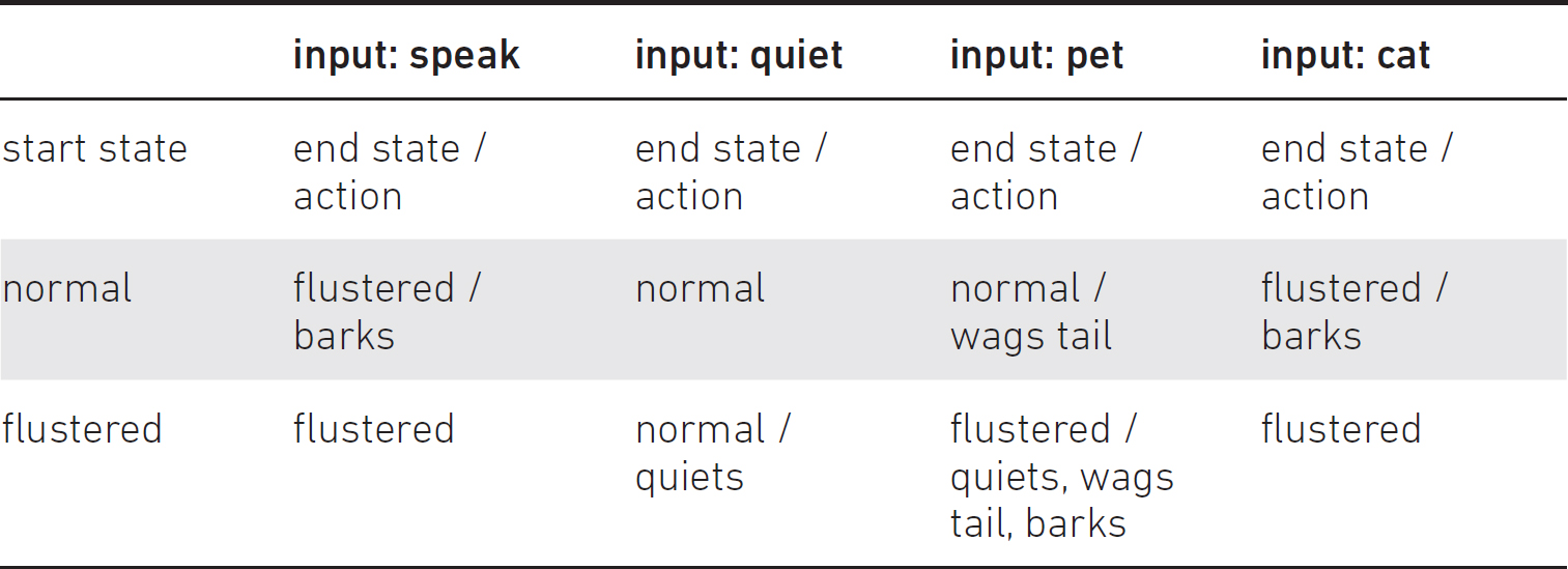
The state diagram and the associated state table are in Figure 6.2 and Table 6.3, respectively.
The state transition table (Table 6.3) shows some undefined transitions. If the RoboDog barks (the automaton is in state s2), the command ‘speak’ or spotting a RoboCat have nothing to activate. If the RoboDog is in a normal state, the command ‘quiet’ has no effect either. We extend the state machine with null transitions (Table 6.4).
Figure 6.2 State diagram for the ‘RoboDog’ example
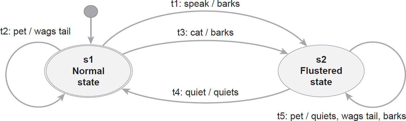
Table 6.3 State–event notation for the ‘RoboDog’ example with undefined transitions

Table 6.4 State–event notation for the ‘RoboDog’ example
Let’s alter the RoboDog specification with the following:
EXAMPLE: ROBODOG (EXTENSION)
When the RoboDog barks and is getting petted, it stops barking, wags its tail for 5 seconds and starts barking again, as before. However, after the third time petting the flustered RoboDog, it stops barking, wags its tail for 5 seconds and then goes quiet.
The state table changes (as shown in Table 6.5) where there are new actions, namely
• a4: PettingNo is set to zero (:= 0), (setzero);
• a5: Increments PettingNo (incr).
Table 6.5 State–event notation for the extended ‘RoboDog’ example
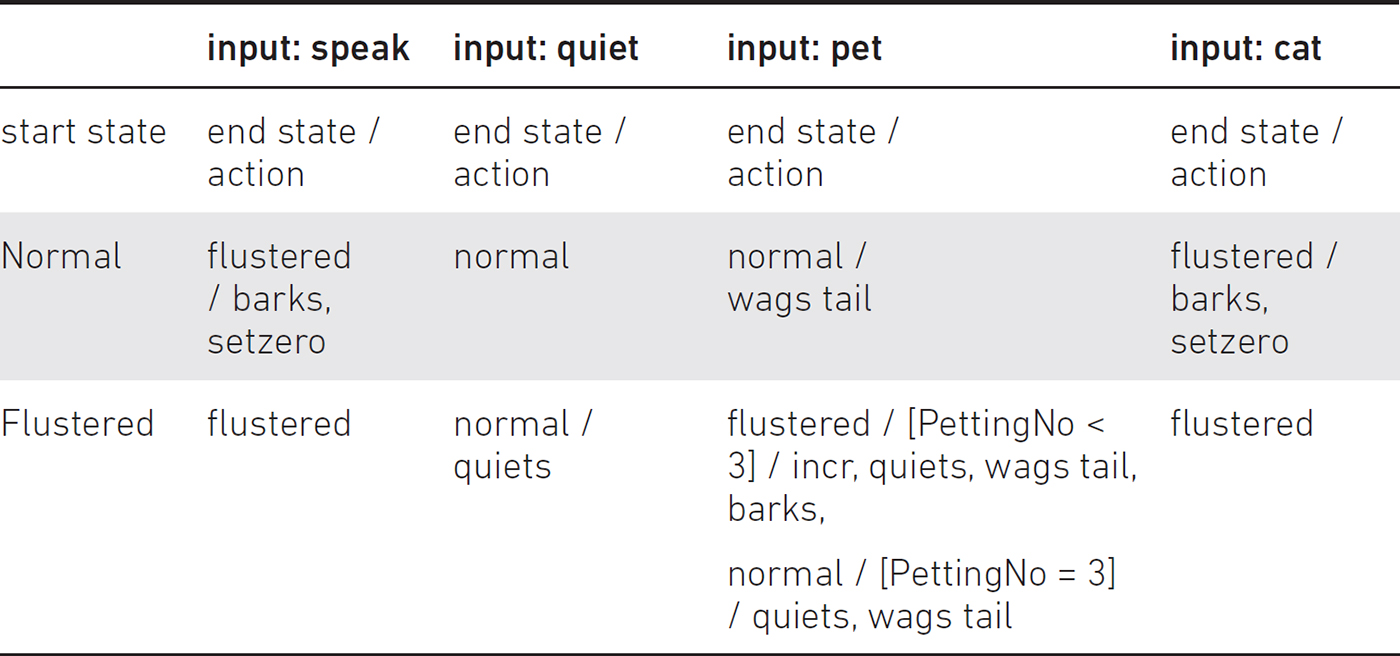
We note that PettingNo should be global for the system and initiated to zero at the beginning (precondition). See the resulting state diagram (Figure 6.3).
Figure 6.3 State diagram for the extended ‘RoboDog’ example

Altogether we have two states, four events and five possible actions. Observe that the guard conditions for the petting number cover the whole domain, that is 0 ≤ PettingNo < 3 or PettingNo = 3; other values are not possible.
VALIDATE YOUR STATE TRANSITION GRAPH
When the state transition graph (or table) has been created the test designer must carefully analyse and validate it.
The following guidelines help in analysing the completeness and consistency of the state transition graph model.
• State, event and action names must be unambiguous and meaningful in the context.
• There must be an initial state and at least one final state in the automaton. If the latter does not exist, the termination condition should be made explicit.
• Every state must be reachable from the initial state (not necessarily in one step).
• Every state shall have at least one ingoing and one outgoing transition except the initial and the final states. (Anther exception can be an ‘error collector’ node. If this rule is violated, the tester has to know why.)
• Every defined event and action shall come up in at least one transition.
• The actions cannot influence the behaviour of the state machine; their implementation does not contain ‘teleports’.
• The state machine shall be complete, that is,
▪ All state/event pairs have a transition. If not, check the specification for correctness. Implicitly given completeness is allowed (null transitions).
▪ The error (exception) handling shall be explicitly or implicitly given.
• The state machine should be minimal (with a minimal number of states) or well hierarchised. Sometimes the latter is more important if it supports human readability better.
Practically speaking:
• Naming conventions are important. For example, a name for an action should refer to an action to be performed (in ‘ing’ form, reading, writing, updating, petting, etc.).
• When there is no initial state then it is not clear when to start.
• When a state is not reachable, then something is missing and so on.
When we test a stateful system (system under test, SUT), sometimes it is desirable to fulfil certain properties:
• Status messages. The tester wants to ask the implementation of the SUT’s current state (without changing its state).
• Reset capability. The tester wants to bring the SUT to the initial state. In automated test execution after a blocking event, it can be useful in continuing the testing. Then, the reset capability can be practical.
• Set-state capability. The tester wants to bring the SUT to any given state.
All of these properties can be present reliably or unreliably. The following checklist extends the previous guidelines:
• Completely specified? The state transition graph is complete if no states, transitions, events and actions are missing.
• Deterministic or non-deterministic? In a given state, the system returns similar or different results for the same input.
• Strongly connected? All nodes are reachable from each node.
• Reduced or minimal? The same behaviour exists with a smaller state machine.
• Reliable/unreliable reset? Or reset capability does not exist?
• Reliable/unreliable status message? Or status message capability does not exist?
• Reliable/unreliable set-state? Or set-state capability does not exist?
Satisfying a test selection criterion, we shall cover the nodes/edges/paths of the state transition graph. Also we have to consider the semantics of the graph (the specification) as well. For example, in the extended RoboDog example, the transition t6 can happen only after petting twice the flustered RoboDog.
There are different fault models available to the stateful systems.
Validating the state machine against control faults
When testing an implementation against a state machine, the following typical control faults should be examined.
• Missing transition (nothing happens as a consequence of an event). In the RoboDog example, if t2 (if the RoboDog is getting petted, it wags its tail for 5 seconds, and remains in a normal state) is missing, then petting the RoboDog has no consequence in the normal state (there is no tail wagging).
• Extra transition. The extra transition may mean incorrect behaviour.
• Incorrect transition (the resulting state is incorrect). For example, if t2 were incorrect (t2 goes from s1 to s2), then by petting the RoboDog two times it would behave incorrectly (the RoboDog starts barking unexpectedly).
• Missing event. The system is unable to handle some events.
• Extra event. The implementation accepts undefined events. Avoiding extra events is especially important for analysing security or safety criteria (trap doors).
• Incorrect event. The system behaves incorrectly. For example, giving the command ‘quiet’ to the RoboDog in the normal state it starts barking (in transition t1 the event ‘speak’ has been changed to ‘quiet’).
• Missing, extra or incorrect action. As a result of a transition, nothing or inappropriate actions happen. For example, the RoboDog begins to wag its tail for the command ‘speak’.
• Missing, extra or incorrect state. These kinds of faults can be interpreted together with transition faults belonging to that state.
TEST SELECTION CRITERIA FOR STATE TRANSITION TESTING
State transition testing is measured mainly for valid transitions. There are many different test selection criteria regarding the transition-based method. First, we explain only the methods, then we show their thoroughness.
Test selection criteria for transition-based models
The examples in this subsection come from Figure 6.2, and we always aim to achieve full (100 per cent) coverage. We use the usual ‘big oh’ notation for describing the time complexities for calculating the tests.
Classical criteria
The following criteria are related to the states, events and transition sequences:
• All-states criterion, in which each state is visited at least once by some test case in the test suite.
▪ The transition sequence t1–t4 is appropriate. The test sequence can be [speak, quiet].
▪ Complexity: O(number of states).
• All-events criterion, in which each event of the state machine is included in the test suite (all events are part of at least one test case).
▪ The test can be [cat, quiet, pet, speak].
▪ Complexity: O(number of events).
• All-actions criterion, in which each action is executed at least once.
▪ The test [speak, quiet, pet] results in the RoboDog barking, quieting and wagging its tail for 5 seconds.
▪ Complexity: O(number of actions).
• All-transitions criterion, in which every transition of the model is traversed at least once (called Chow’s zero-switch coverage) (Chow, 1978). It implies (subsumes) all-events, all-states and all-actions criteria.
▪ The transition sequence t1-t5-t4-t3-t4-t2 is appropriate, for which the test is [speak, pet, quiet, cat, quiet, pet].
▪ Complexity: O(number of transitions).
Considering the extended RoboDog example (Figure 6.3), we need a different test for the same criterion: [pet, cat, quiet, speak, pet, pet, pet]. Here we used an EFSM, hence, the time complexity depends on the maximal boundary values of the guard condition variables as well.
• All-transition-pairs criterion (called Chow’s one-switch coverage), in which every pair of adjacent transitions are traversed at least once.
▪ The following two transition sequences satisfy the criteria: t2-t2-t1-t4-t1-t5-t4-t3-t5-t4 and t3-t4-t2-t3-t4, for which the tests are {[pet, pet, speak, quiet, speak, pet, quiet, cat, pet, quiet], [cat, quiet, pet, cat, quiet]}.
▪ Complexity: O(transitions2).
• All-n-transitions criterion (called Chow’s n-switch coverage), in which every transition sequence generated by n+1 consecutive events is exercised at least once. The all-n-transitions criterion implies (subsumes) all-(n-1)-transitions criteria.
▪ Complexity: O(transitionsn+1). Observe that this is exponential in the number of transitions.
Besides the complexity, there is another shortcoming of this criterion. Namely, it produces too many infeasible paths. It is important to note that in practice most of the faults regarding consecutive states in a state machine are mainly 1-switch or 2-switch faults; 3 or more switch faults are very rare.
• All configurations criterion, in which parallel systems are modelled in a way that every configuration is visited at least once. A configuration is a ‘snapshot’ of the active states of the parallel processes. If no parallelism exists, then it is equivalent to the all-states coverage.
The following criteria are related to traversing the possible loops:
• All loop-free paths criterion, in which every loop-free path is traversed at least once.
▪ Complexity: O(states × log(transitions)) (spanning tree searching).
• All-round-trip paths criterion. We need some definitions: a simple path is a path in which any node cannot appear more than once except maybe the starting and the ending nodes. A prime path is a simple path that does not appear as a sub-path of any other simple path. A round-trip path is a prime path of non-zero length that starts and ends with the same node. A complete round-trip coverage means that every round-trip path for each reachable node should be taken.
• All-one-loop paths criterion, in which all loop-free paths are traversed plus all the paths that loop once.
• All-path criterion. Every path should be traversed in the state diagram at least once. Similar to exhaustive testing, in general, it is impossible to satisfy.
The following is not really a criterion, but it is a useful non-deterministic technique for traversing a graph.
• Random walking. A random walk is a trajectory that consists of successive random steps in the graph model. For more details see the GraphWalker section in Chapter 13.
We have to discuss the ‘minimality’ of the constructed sets. Before optimising the test sets, a target function should first be determined. This can be the expected running time, some restrictions on the number of the test cases, the number of transitions in a test case, the average length of the tests and so on. This optimisation can be hard, as with pairwise testing, whose task is nondeterministic polynomial (NP)-complete (Lei and Tai, 1998). In practice, however, it is enough to approach close to the optimum value.
Please do not underestimate the importance of the random walk coverage. Many test design automation tools use this approach since for small–medium state transition graphs it works effectively (the GraphWalker section in Chapter 13). For simpler state diagrams the test cases can even be created manually.
All-transition-state and all-transition–transition criteria
Unfortunately, simple criteria are sometimes weak; strong criteria may lead to exponential explosion. The main question is as follows: Is there any criterion between them that is both reliable and manageable? Here we introduce two criteria, which we think of as both reliable and ‘cheap enough’ to use in practice.
The rationale behind these criteria is the following:
1. When there is a faulty computation in an action through a transition t, and the erroneous data is used later at a transition belonging to the state s, then the program fails. Therefore, it is reasonable to test each transition-state pair (t, s).
2. Let’s assume that erroneous data is defined in a transition; however, the same data is defined correctly in another transition t. If a test case traverses t, avoids the other one, and is used later at an action belonging to s, then the bug remains undetected. Therefore, we shall omit the path from t to s, and we will denote these paths by (!t, s).
3. Now let’s assume that there is a guard condition related to a transition t. The guard condition determines a boundary value and we shall test this boundary with ON and OFF points by traversing the transition t as many times as is needed. For example, in our TVM we can buy a maximum of 10 tickets. We shall test the boundary point by trying to traverse the transition beyond the limit, that is 11 times.
With these three requirements the first test selection criterion is the following:
ALL-TRANSITION-STATE CRITERION
For a given transition t let’s denote the set of all reachable states by RS(t) for which there is a path via the transition t to any element of RS(t). Then, satisfying the criterion means that
1. The test set must cover at least one path via t to S for all transition t and S ϵ RS(t),
2. There is at least one path to all S ϵ RS(t) that does not include the transition t (if possible),
3. When there is a boundary value guard condition for a transition t in path P then P should be extended in a way that the number of traversing t reaches the boundary value of that guard condition (if feasible). Informally, the given transition should be traversed multiple times, till the boundary value of the guard condition is reached.
Note that reachability mainly means available paths in the state transition graph, but may mean feasibility (executability) in the case of test generation. Note as well that satisfying the all-transition-state criterion also satisfies the all-transitions criterion.
Now let’s consider our RoboDog example and investigate the test (steps) to satisfy this criterion. The graph is strongly connected; moreover, by deleting any transition except t4, it remains strongly connected. Hence, the sequence
s1-t2-s1-t1-s2-t5-s2-t4-s1-t3-s2-t4-s1
covers the (t, s) paths for all transition t and s ϵ RS(t), and the sequences
s1-t1-s2-t4-s1, s1-t3-s2-t4-s1
cover the (!t, s) paths. The appropriate test set is
{[pet, speak, pet, quiet, cat, quiet], [speak, quiet], [cat, quiet]}.
Sometimes even this test selection criterion is weak. For a stronger criterion, we have to consider each (t, t’) pairs. The related definition is the following:
ALL-TRANSITION–TRANSITION CRITERION
For a given transition t let’s denote the set of all reachable transitions from t by RT(t) for which there is a path via the transition t to any element of RT(t). In the case of looping, t ϵ RT(t). Then, the coverage means that
1. The test set must cover at least one path via t to t’ for all transition t and t’ ϵ RT(t),
2. There is at least one path to all t’ ϵ RT(t) that does not include the transition t (if possible),
3. When there is a guard condition for transition t in path P then the path should be extended in a way that the number of traversing t reaches the boundary value of that guard condition (if feasible).
Complexity: without the third condition, the number of test cases is quadratic in the worst case since we shall cover pairs of transitions. The existence of boundaries may increase the complexity proportionally to their maximal value.
How can we satisfy this stronger criterion for the extended RoboDog? Since the state transition graph of the RoboDog is Eulerian, that is we start from s and traversing each edge only once we can go back to s, the path
s1-t1-s2-t4-s1-t2-s1-t3-s2-t5-s2-t4-s1-t2-s1-t1-s2-t4-s1-t3-s2-t5-s2-t4-s1
satisfies the first criterion, and partly the second, that is
(!t1, t1), (!t2, t1), (!t3, t1), (!t4, t1), (!t5, t1), (!t2, t4), (!t3, t4), (!t4, t4), (!t5, t4), (!t2, t2), (!t3, t2), (!t5, t2), (!t3, t3), (!t5, t3), (!t5, t5).
The rest can be satisfied with the paths
s1-t2-s1-t3-s2-t4-s1-t1-s2-t4-s1, s1-t3-s2-t5-s2-t4-s1 and s1-t1-s2-t5-s2-t4-s1
since in these cases the following pairs are valid:
(!t1, t2), (!t4, t2), (!t4, t3), (!t1, t3), (!t2, t3), (!t1, t4), (!t1, t5), (!t2, t5), (!t4, t5), (!t3, t5).
The test set is
{[speak, quiet, pet, cat, pet, quiet, pet, speak, quiet, cat, pet, quiet], [pet, cat, quiet, speak, quiet], [cat, pet, quiet], [speak, pet, quiet]}.
Recall that the Chow coverage test set becomes exponentially larger with growing n. We note that the all-transition-state and the all-transition–transition criteria measures may serve as a bridge between the linearity and the exponentiality. These two criteria aim at examining defects that cannot be unfolded by Chow’s switching criteria, that is when the defects are ‘far away’ from each other. The boundary value guard is related to boundary value analysis.
Thoroughness of the criteria
Recall that the extended RoboDog state transition graph contains two states, four events, and six transitions. The extra precondition of this state transition diagram is that the global variable PettingNo is defined as zero. Let’s suppose that the behaviour shown in Figure 6.4 has been implemented.
There are three changes (faults) compared to the specified behaviour. In transition t3 there is a missing initialisation, and instead of three, after the fourth time petting, the flustered RoboDog stops barking, wags its tail and goes quiet (these faults are in the transitions t5 and t6). Of course, the black-box tester does not know about this. Suppose that the tester designs the test cases for satisfying the all-states, all-events, all-actions, all-transitions criteria according to the model shown in Figure 6.3.
Figure 6.4 Programmed behaviour of the ‘RoboDog’. The difference from the specified behaviour is underlined

Table 6.6 shows a simple short test. The test does not show any faults. The faults are in combination, that is the missing initialisation causes RoboDog to quiet at step 8. OK, we think, very good, let’s check the 1-switch criterion by Chow. The clever tester observes that the transition pairs t1–t6 and t3–t6 are impossible (because of the specification), therefore they omit them from the test design. To spare time, the tester divides the previous test into two parts: ShortTest = [t2, ShorterTest]. Then, their result is the following test:
Table 6.6 Short test for the extended ‘RoboDog’ example

{[ShortTest-ShorterTest-t3-t4], [t2-t3-t4-t1-t4-t2], [ShorterTest-t2]}.
It is easy to check that this test set fulfils the 1-switch coverage criteria, but does not find the faults. The reason is that we have a 2-switch fault, hence, only the 2-switch criteria would be able to find it.
Kuhn et al. (2008) determined that up to 97 per cent of software faults can be detected by at most two variables interacting. These criteria consider pairs, which influence each other. Chow’s switch coverage considers only adjacent transitions, but erroneous influence may come from remote transitions as well. The all-transition-state criterion considers arbitrary (transition, state) pairs; the all-transition–transition criterion arbitrary (transition, transition) pairs. The method could be extended to triples, but pairs are usually enough.
Let’s summarise why the proposed criterion is useful. Regarding EFSMs, in some cases, guard condition variable assignments (initialisations) are in the wrong places. To detect this problem, we should cover an execution path excluding a transition with this assignment. Traversing every (!t, s) or (!t1, t2) will reveal the bug. Considering the last criterion, guard condition boundaries should be handled with boundary value analysis techniques.
EXAMPLE: COLLATZ CONJECTURE
Finite-state machines are used to model complex logic in dynamic systems, such as automatic transmissions, robotic systems and mobile phones. This complex logic includes operations like scheduling tasks, supervising how to switch between different modes of operation, recovery logic and so on.
The following example presents complex logic with elementary operations. We show how to model it with a state transition graph, and we analyse some loop-related test selection criteria.
EXAMPLE: COLLATZ
The Collatz conjecture concerns a sequence in number theory defined as follows: starting with any positive integer n, each term is obtained from the previous term as follows: if the previous term is even, the next term is half of the previous term. If the previous term is odd, the next term is 3 times the previous term plus 1. The conjecture is that no matter what the value of n is, the sequence will always reach 1. We checked the validity of the conjecture for 2, 3, 4, 5, by hand, and for those cases the computation terminates. We model the computations with a state machine.
Preconditions: there is a global integer variable n, initially set to zero. The variable n can arbitrarily be large. The input is a positive integer.
States:
• s1: Initial state;
• s2: Even state;
• s3: Odd state;
• s4: Final state.
• e1: Getting the input;
• e2: Changing the value of n.
Output (action):
• Result: print(‘the process terminates’).
Transitions:
• t1: e1 / [input is odd] / n := input;
• t2: e2 / [n = 1 OR n = 3 OR n = 5] / Result;
• t3: e1 / [input is even] / n := input;
• t4: e2 / [n = 2 OR n = 4] / Result;
• t5: e2 / [n ≠ 1 AND n ≠ 3 AND n ≠ 5] / n := 3n + 1;
• t6: e2 / [n ≠ 2 AND n ≠ 4 AND n := n/2 is odd] / <>;
• t7: e2 / [n ≠ 2 AND n ≠ 4 AND n := n/2 is even] / <>.
The Collatz machine is in Figure 6.5.
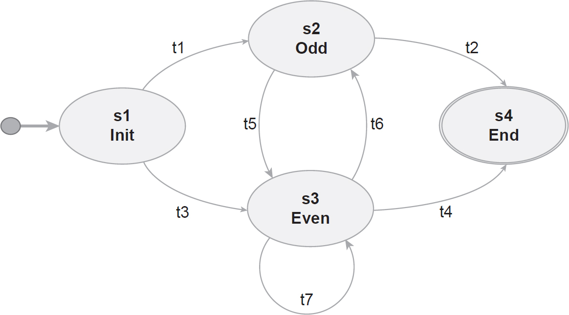
Let’s check the functioning. When the input is 1, 3 or 5 the processing goes through s1-t1-s2-t2 and the output is a message about termination. When the input is 2 or 4, the processing is via s1-t3-s3-t4 and there is a termination message again. Let the input be the magic number 42. Then the processing is the following: s1-t3(n = 42)-s3-t6 (n = 21)-s2-t5(n = 64)-s3-t7(n = 32)-s3-t7(n = 16)-s3-t7(n = 8)-s3-t7(n = 4)-s3-t4 and the output is the termination message. The termination was checked for integers up to 87 × 260 by Roosendaal (2018).
The test data 2 (traversing t3-t4) and 3 (traversing t1-t2) traverses all loop-free paths since t1-t5-t4 and t3-t6-t2 are impossible to get around without looping. Let’s analyse the all-round-trip paths criterion. The only simple paths in the graph are t1-t2, t3-t4, t3-t6-t2 and t1-t5-t4. Hence, the tests for this criterion are identical to the all-loop-free paths tests. To get tests for the all-one-loop path criterion, we have to add one loop for the possible loop-free paths. The transition sequence t3-t7-t4 is reliable; the test data is (for example) 8. The sequence t3-t6-t5-t4 is unreliable. The sequence t3-t7-t6-t2 is reliable with test data = 6. The sequence t1-t5-t7-t4 is unreliable as well as the sequence t1-t5-t6-t2.
WHEN MULTIPLE TECHNIQUES ARE USED TOGETHER
This may be a surprise, but it’s difficult to find any description or examples on how to apply more test design techniques together. Here is a short introduction where we demonstrate using multiple techniques through our example. Usually we combine two techniques, therefore we will demonstrate this case; however you can easily extend it.
• Make the test design for the two techniques separately.
• Select the one that has more test cases.
• Map the test cases of the other technique to these test cases.
• If some test cases cannot be mapped, try to refactor the test cases for better mapping.
• Map the refactored test cases again.
• Validate the test cases.
In this section we consider a specific, simplified part of the specification ‘Two lifts in a 10-storey building’ described in Chapter 4. The slightly reduced specification can be tested independently from the other parts. The most important requirement in this case says that all the guests should be served (sooner or later). For example, if the lift goes down from the upper floor, and the guest − who called it first − is standing on the fifth floor, but after a few seconds a family calls the lift at the sixth floor, then the lift may become full, and the guest at five cannot enter. The specification guarantees that a similar situation cannot happen (except when the lifts never become empty, but this case is unrealistic).

I have frequently noticed when checking out from a hotel with my luggage that some lift specifications consider cost-effectiveness more important than guests. For instance, the lifts went first to the guests on the higher floors, then collected the other guests on their way down. Unfortunately, because of the huge morning traffic, the lifts almost always became full at the higher levels, and I could not enter. After 2–3 attempts I changed my mind and took the stairs.
Here we have omitted some of the steps in the original specification (see Chapter 4).
F-CMC-1 If both lifts are vacant and a user requests one, then the closer lift will always start in the caller’s direction. In the case of equality, Lift1 is chosen.
F-CMC-2 If one of the lifts is vacant and the other one is moving, then the vacant one starts for the requester.
F-CMC-3 When no lift is available then the user request is scheduled.
F-CMC-4 When a lift becomes vacant, the oldest pending request must be handled first.
F-CMC-5 The serving order depends on the location of the lifts, on their moving direction and on their request queues.
F-CMC-6 The non-empty lift stops for users when an up/down call is received from them while the lift is moving up/down as well and approaching the user.
F-CMC-7 The empty lift goes for the guest first in the queue and does not stop for other guests.
Here we do not consider priorities.
This is a good example as different test design techniques are applied together. Clearly, the model is reactive since it contains states such as vacant, moving or standing lifts (waiting for the guests to leave and/or enter).
For this example, we show you step by step how to design test cases involving STT, EP and BVA together. The first step is to create the state transition diagram.
Preconditions: the starting state is when both lifts are vacant.
States:
• s1: Lift1, Lift2 vacant;
• s2: Only Lift1 is vacant;
• s3: Only Lift2 is vacant;
• s4: Lift1 is moving;
• s5: Lift2 is moving;
• s6: Lift1 is standing;
• s7: Lift2 is standing.
• e1: Guest calls from outside the cabin (up/down);
• e2: Guest requests from inside the cabin in Lift1 (pushing target level number);
• e3: Guest requests from inside the cabin in Lift2 (pushing target level number);
• e4: Lift1 weight control notices that all guests leave it (empty lift signal);
• e5: Lift2 weight control notices that all guests leave it (empty lift signal).
Note that if not all the guests leave a lift, then there shall be a guest request. Here we do not consider the non-functional requirement when a guest is not able to get out or press a button. Remember an outside guest calls a lift; a guest inside the cabin requests the lift to stop at a chosen floor.
Outputs:
• o1: Lift1 starts according to the inside request, or if it is empty, then to the floor of the oldest pending guest;
• o2: Lift2 starts according to the inside request, or if it is empty, then to the floor of the oldest pending guest;
• o3: Lift1 stops and opens door, the queue of the pending callers is updated, if needed;
• o4: Lift2 stops, opens door, the queue of the pending callers is updated, if needed;
• o5: Lift1 opens door, the queue of the pending callers is updated, if needed;
• o6: Lift2 opens door, the queue of the pending callers is updated, if needed.
Transitions:
• When Lift1 and Lift2 are vacant, and there is an outside guest call (first in the queue) closer or equal to Lift1,
▪ t1: Lift1 serves the guest by moving for them if the caller and Lift1 are on different levels (o1),
▪ t2: Lift1 serves the guest by opening its door if they are at the same level (o5).
Lift2 remains vacant in both cases.
• When Lift1 and Lift2 are vacant, and there is an outside guest call (first in the queue) closer to Lift2, then
▪ t11: Lift2 serves the guest by moving for them if they are on different levels (o2), Lift1 remains vacant.
• t3: When Lift1 is approaching the next floor and there is an acceptable guest call then the lift stops and opens door (o3),
• t13: When Lift2 is approaching the next floor and there is an acceptable guest call in the request database, then the lift stops and opens door (o4),
• t4: When Lift1 is approaching the next floor and there is a guest request to that floor, the lift stops and opens door (o3),
• t14: When Lift2 is approaching the next floor and there is a guest request to that floor, the lift stops and opens door (o4),
• t5: When (the non-empty) Lift1 is standing and there is a guest request in it, then Lift1 starts and goes towards the requested floor (o1),
• t15: When (the non-empty) Lift2 is standing and there is a guest request in it, then Lift2 starts and goes towards the requested floor (o2),
• t6: When all guests leave Lift1 (no guest request remains), it is vacant,
• t16: When all guests leave Lift2 (no guest request remains), it is vacant,
• When only Lift1 is vacant, and there is an outside guest call non-acceptable for Lift2, then
▪ t7: Lift1 serves the guest by moving for them if the caller and Lift1 are on different levels (o1),
▪ t8: Lift1 serves the guest by opening its door if they are on the same level (o5),
• When only Lift2 is vacant, and there is an outside guest call non-acceptable for Lift1, then
▪ t17: Lift2 serves the guest by moving for them if the caller and Lift2 are on different levels (o2),
▪ t18: Lift2 serves the guest by opening its door if they are on the same level (o6),
• t9: When Lift1 is vacant, and Lift2 becomes empty, Lift1, Lift2 are vacant,
• t19: When Lift2 is vacant, and Lift1 becomes empty, Lift1, Lift2 are vacant.
Note that ‘acceptable call’ means that:
• If the lift is non-empty then:
(1) a guest (outside the cabin) pushed UP/DOWN at a level; and
(2) the lift is moving towards the guest.
• If the lift is empty then the only acceptable call is the first pending call.
The system is concurrent since ‘it includes a number of execution flows that can progress simultaneously, and that interact with each other’ (Bianchi et al., 2017). Extension of state diagrams are Harel (and Unified Modelling Language (UML)) statecharts (see the ‘Theoretical background’ section later in this chapter). Concurrency in statecharts can be shown explicitly using ‘fork’ and ‘join’. A fork is represented by a bar with more outgoing arrows; a join is represented by a bar with more incoming arrows.
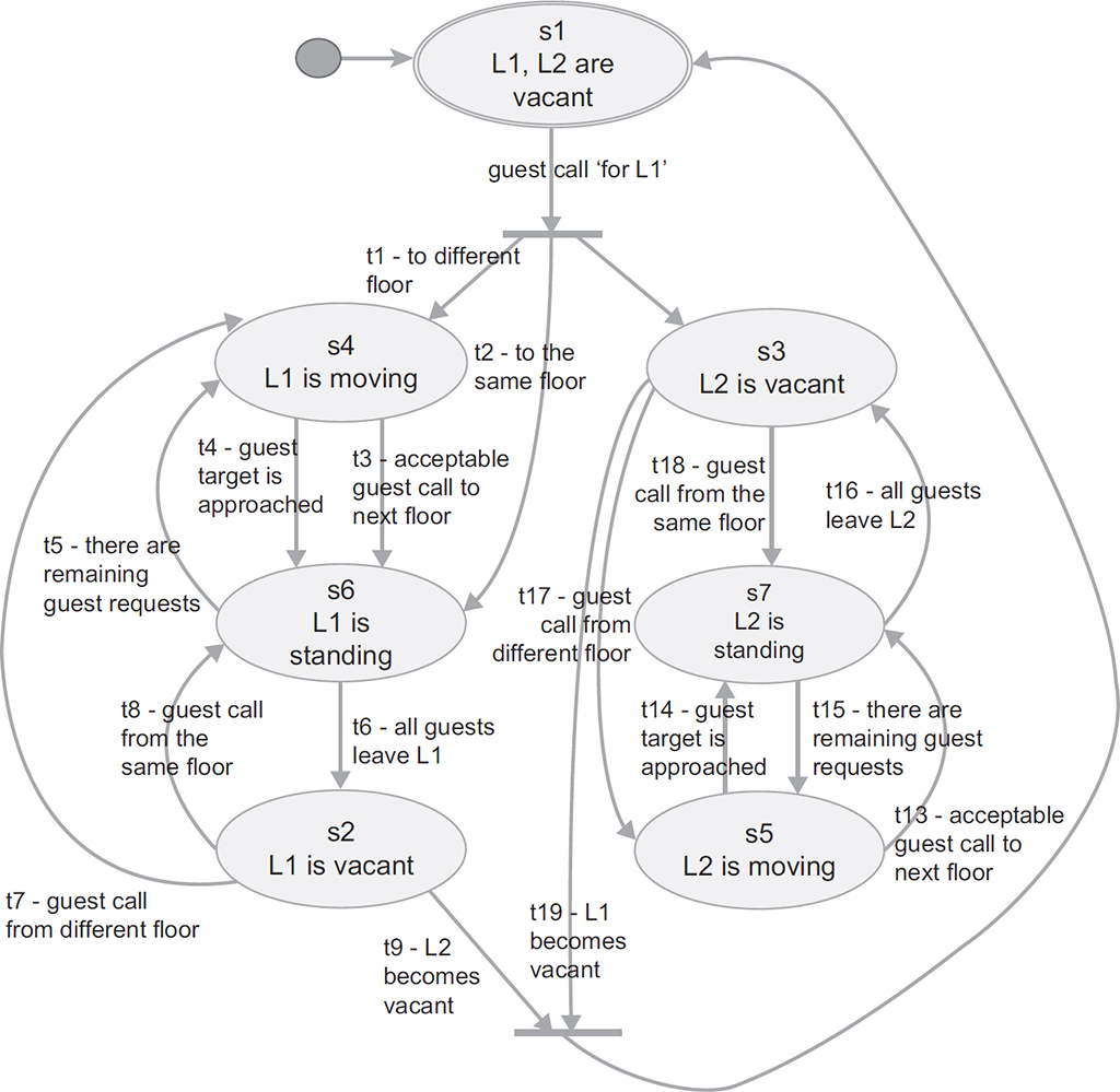
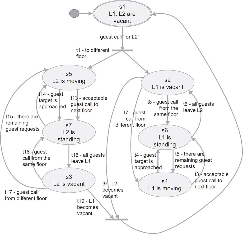
Here we have two parallel sub-systems: one for Lift1 and the other for Lift2. For simplicity we cut the state transition diagram into two parts (Lift1 and Lift2 are L1 and L2, respectively, see Figures 6.6a and 6.6b). The figures are almost symmetric (t2 does not have a ‘pair’).
Figure 6.6a State transition graph for ‘Two lifts in a 10-storey building’ – Lift1
Let’s consider some examples.
• Lift1 is non-empty and moving upwards approaching floor 3. Lift2 is vacant. The first pending call is upwards at floor 5. Lift2 will start.
• Lift1 is non-empty and moving upwards approaching floor 3, Lift2 is not vacant and moving down from floor 9. The first pending call is up at floor 5, the second is down at floor 3 and the third is up at floor 4. Lift1 will stop at floor 4, then at floor 5 but it will not stop at floor 3. Lift2 will stop at floor 3.
Up to now we have not considered testing concurrent systems. There are several test selection criteria for concurrent systems (Bianchi et al., 2017). Here we consider a very simple criterion that requires all states to be held in parallel. For example, if Lift1 is moving, then Lift2 shall (1) stand (2) move, (3) remain vacant.
Figure 6.6b State transition graph for ‘Two lifts in a 10-storey building’ – Lift2
We can extend the all-state-transition criterion for concurrent systems in a way that each (transition, state) pair is executed for all concurrent execution flows.
According to this criterion we have the following test steps for Figure 6.6a, and remember that the two sub-diagrams are similar as L1 → L2 and L2 → L1.
The test path for the concurrent case (ST-Tpath2) is described by two parallel sequences containing the states such as s6 L1 is standing and transitions such as t5 – there are remaining guest requests.
ST-Tpath1: simple, see Table 6.7.
ST-Tpath2: both lifts are vacant at the beginning and the end of this test path, see Table 6.8.
Table 6.7 State transition test for ‘Two lifts in a 10-storey building’, ST-Tpath1
s1 L1, L2 are vacant |
t1 – to different floor |
s4 L1 is moving t4 – guest target is approached |
s6 L1 is standing t5 – there are remaining guest requests |
s4 L1 is moving t4 – guest target is approached |
s6 L1 is standing t6 – all guests leave L1 |
s1 L1, L2 are vacant |
Table 6.8 State transition test for ‘Two lifts in a 10-storey building’, ST-Tpath2
Lift1 |
Lift2 |
s1 L1, L2 are vacant t1 – to different floor |
|
s4 L1 is moving t3 – acceptable guest call to next floor |
s3 L2 vacant |
s6 L1 is standing t5 – there are remaining guest requests |
|
s4 L1 is moving t3 – acceptable guest call to the next floor |
|
s6 L1 is standing t5 – there are remaining guest requests |
|
s4 L1 is moving |
|
t4 – guest target is approached |
t18 – guest call from the same floor |
s6 L1 is standing |
s7 L2 is standing |
t6 – all guests leave L1 |
t15 – there are remaining guest requests |
s5 L2 is moving |
|
|
t14 – guest target is approached |
t7 – guest call from different floor |
s7 L2 is standing |
s4 L1 is moving |
t16 – all guests leave L2 |
t3 – acceptable guest call to next floor |
s3 L2 vacant |
s6 L1 is standing |
|
t5 – there are remaining guest requests |
t17 – guest call from different floor |
s4 L1 is moving |
s5 L2 is moving |
t4 – guest target is approached |
t13 – acceptable guest call to next floor |
s6 L1 is standing |
s7 L2 is standing |
t6 – all guests leave L1 |
t15 – there are remaining guest requests |
s2 L1 is vacant |
s5 L1 is moving |
|
t13 – acceptable guest call to the next floor |
|
s7 L2 is standing |
|
t15 – there are remaining guest requests |
t8 – guest call from the same floor |
s5 L2 is moving |
s6 L1 is standing |
t14 – guest target is approached |
t5 – there are remaining guest requests |
s7 L2 is standing |
s4 L1 is moving |
t16 – all guests leave L1 |
t4 – guest target is approached |
s3 L2 is vacant |
s6 L1 is standing |
|
t6 – all guests leave L1 |
|
s2 L1 vacant |
t19 – L1 becomes vacant |
t9 – L2 becomes vacant |
|
s1 L1, L2 are vacant |
|
Here, the left column contains the movement of Lift1 (L1) and the right one contains the movement of Lift2 (L2). Lift1 is vacant four times (1) at the beginning, (4) at the end and (2), (3) to test guest calls from different floors (2), and a guest call from the same floor (3). Lift2 is vacant three times (1) for testing guest calls from the same floor, (2) testing a guest call from different floors and (3) when both lifts become vacant. The vacancies happen at different times, hence the concurrent test selection criterion is satisfied.
We can see that except for t2, all the transitions are covered. We traverse ST-Tpath2, then ST-Tpath4 in a similar way, which result in the ‘traditional’ all-state transition criterion being satisfied. This is because in traversing ST-Tpath4, all the states are covered after t2 and all other transitions in ST-Tpath2. We have the 4th test path ST-Tpath3, which is symmetric with ST-Tpath1.
Now let’s consider the EP and BVA part. We have two lifts, Lift1 and Lift2. The third ‘participant’ is the guest calling them. There are several different locations of this {Lift1, Lift2, guest} triple. There are several elements of this triple; however, we can classify them. For example, the cases (Lift1=2, Lift2=9, guest=3) are similar to (Lift1=2, Lift2=8, guest=4) as in both cases Lift1 shall start. In this way the elements in the triple can be classified into four EPs:
EP1: Guest is in between the lifts and Lift1 is not further than Lift2 from the guest.
EP2: Lift1 is between the guest and Lift2 (including the case when Lift1 and Lift2 are on the same level) – obviously, Lift1 is not further.
EP3: Guest is in between the lifts and Lift2 is closer.
EP4: Lift2 is between the guest and Lift1 – obviously, Lift2 is closer.
Let’s extend the EPs with boundary values. Though three points are required for each EP, because of overlap, eight test cases are enough. The test inputs are shown in Table 6.9.
Table 6.9 BVA test input for ‘Two lifts in a 10-storey building’, ST-Tpath1

There are also equivalence partitions related to the guests: whether they can be picked up or not by a moving lift. These EPs shall be tested in a way that if a guest cannot be picked up, then the other lift shall start. There are other EPs to test whether the moving lift stops or the other will start:
EP11: Non-empty Lift1 is approaching up/down to the guest who pushed up/down – Lift1 stops.
EP12: Non-empty Lift1 is approaching up/down to the guest who pushed up/down – vacant Lift2 starts.
EP13: Non-empty Lift1 is moving up/down, the guest pushed up/down, but Lift1 is moving away from this guest – vacant Lift2 starts.
EP14: Lift1 is empty and approaching the guest who first called it. Another guest called a lift – Lift2 starts.
EP15: Non-empty Lift2 is approaching up/down to the guest who pushed up/down – Lift2 stops.
EP16: Non-empty Lift2 is approaching up/down to the guest who pushed up/down – vacant Lift1 starts.
EP17: Non-empty Lift2 is moving up/down, the guest pushed up/down, but Lift2 is moving away from this guest – vacant Lift1 starts.
EP18: Lift2 is empty and approaching the guest who first called it. Another guest calls a lift – Lift1 starts.
Note that ‘approaching’ floor x means moving to floor x and possibly standing between moving to y and moving from y to x. We do not consider the EPs when one lift is vacant, and the guest is on the same or different level. This is because we have covered these cases by covering the related transitions.
The next step is to combine the test design techniques. Here we start from STT and map a BVA test to it. We design our first test case based on ST-Tpath2 (see Table 6.10). Here the events occurring at a state are to the right of the state, for example Lift1 is standing at (floor) 7 when Guest1 pushes (floor) 1.
Table 6.10 BVA test input for ‘Two lifts in a 10-storey building’, ST-Tpath2
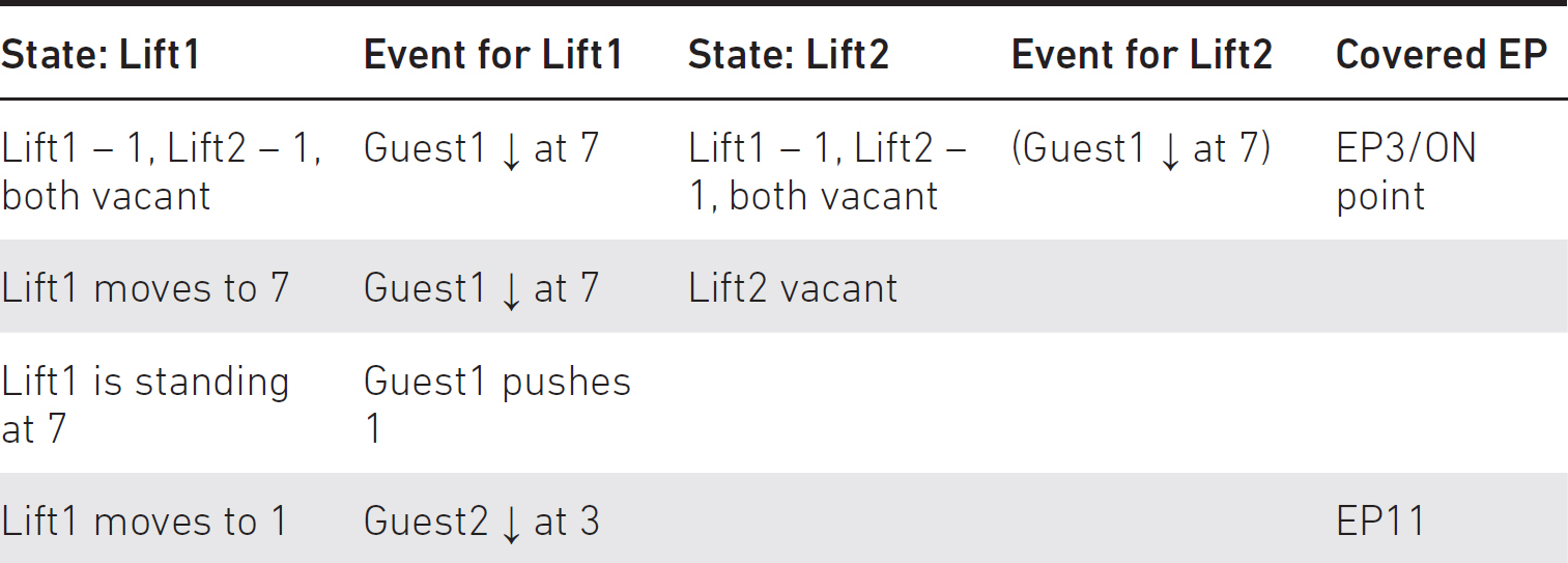

Besides the EP3 ON point, we have covered EP11, EP12, EP15 and EP16. We can easily cover the EP1 ON point, EP13, EP14, EP17 and EP18 in ST-Tpath4. We can cover the remaining two ON points by ST-Tpath1 and ST-Tpath2. Finally, we should test the remaining four IN points by four simple test cases avoiding concurrency.
Summarising, when combining more techniques, a possible process is the following:
1. Design the test cases for the selected techniques separately.
2. Work out a plan on how to integrate the tests from the different techniques.
3. Select the larger set of test cases related to a test design technique, and map the test cases of the other technique to them (if possible).
4. Design additional integrated test cases for which the mapping is not possible.
5. Review and validate the result.
STATE TRANSITION TESTING IN TVM EXAMPLE
Let’s consider the following part of the example TVM specification.
EXAMPLE: TVM TICKET SELECTION
There are three types of tickets:
a. Standard ticket valid for 75 minutes on any metro, tram or bus line.
b. Short distance ticket valid within five stations on a single line of any metro, tram or bus.
c. 24-hour ticket for unlimited metro, bus and train travel for 24 hours from validation.
The price of the tickets can be modified, currently (a) is EUR 2.10, (b) is EUR 1.40 and (c) is EUR 7.60.
Selecting tickets: the customer can buy tickets of one type only. If all the amounts of ticket types are zero, then any of them can be increased. After that, the ticket type with non-zero can be increased or decreased by clicking on ‘+’ or ‘-’. The maximum number of tickets to be bought is 10. ‘+’ and ‘-’ are unavailable when the number of tickets is 10 or 0, respectively. If the selected amount of tickets is greater than 0, then the buying process can start.
We model the ticket selection process of the TVM with a state transition graph. The first step is to create the state transition diagram. Usually, this is the simplest task. To do this, you must read the specification at least twice, maybe more times, and very carefully. You cannot create the correct graph until you really know this part of the specification.
It is not enough to simply understand the specification on a basic level; it needs to be understood in depth!

If you know it well, you can start the design.
First, make a draft version by considering all the states, events and actions, then the ‘forward’ and ‘backward’ transitions one by one. The design is always an iterative process – it is not a problem if the draft version is not complete or is inconsistent. Approach the final version step by step. Finally, validate the graph.
Precondition: the TVM shows the initial ticket selection screen. The number of tickets is set to zero (NrT := 0) and the ticket type value is empty (TicketType := ‘ ’).
States:
• s1: Initial state (Init);
• s2: Standard ticket selection (Stan);
• s3: Short distance ticket selection (Short);
• s4: 24-hour ticket selection (24h);
• s5: Payment (final state) (Pay).
Input (events):
• e1: Increasing the number of standard tickets (incStan);
• e2: Increasing the number of short distance tickets (incShort);
• e3: Increasing the number of 24-hour tickets (inc24);
• e4: Decreasing the number of standard tickets (decStan);
• e5: Decreasing the number of short distance tickets (decShort);
• e6: Decreasing the number of 24-hour tickets (dec24);
• e7: Selecting for payment (selectPay).
Output (actions):
• a1: Increments the number of standard tickets (NrT := NrT + 1)(Stan+);
• a2: Increments the number of short distance tickets (NrT := NrT + 1)(Short+);
• a3: Increments the number of 24-hour tickets (NrT := NrT + 1)(24+);
• a4: Decrements the number of standard tickets (NrT := NrT – 1)(Stan-);
• a5: Decrements the number of short distance tickets (NrT := NrT – 1)(Short-);
• a6: Decrements the number of 24-hour tickets (NrT := NrT – 1)(24-);
• a7: Goes to the payment screen (payment), passing the global data value NrT.
• t1: incStan / Stan+;
• t2: incShort / Short+;
• t3: inc24 / 24+;
• t4: decStan / [NrT = 1] / Stan-;
• t5: decShort / [NrT = 1] / Short-;
• t6: dec24 / [NrT = 1] /24-;
• t7: incStan / [NrT < 10] / Stan+;
• t8: incShort / [NrT < 10] / Short+;
• t9: inc24 / [NrT < 10] / 24+;
• t10: decStan / [NrT > 1] / Stan-;
• t11: decShort / [NrT > 1] / Short-;
• t12: dec24 / [NrT > 1] / 24-;
• t13: selectPay / <A7, TicketType := ‘Standard’>;
• t14 – selectPay / <A7, TicketType := ‘Short Distance’>;
• t15 – selectPay / <A7, TicketType := ‘24 hour’>.
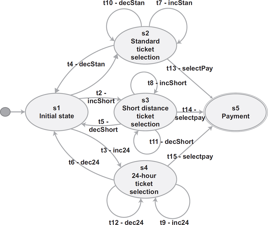
The state transition graph of the TVM can be seen in Figure 6.7.
The next task is to choose the test selection criterion and to create the test cases based on the graph. In our case, the all-transition-state criterion seems to be the most promising. The others have either too weak fault-detection capabilities or need too many test cases.
We can see that the graph is symmetric for the ticket types available to buy. Clearly, for all transitions t, except t13, t14 and t15, the reachable states are RS(t) = {s1, s2, s3, s4, s5}. The following three tests cover those (t, s) pairs for which from each transition t there is a path to all the elements of RS(t). For clarity, we use the names of the transitions and the abbreviation of the states as follows: St, 24, Short, Success and Init:
Tpath1 = Init – incStan – St – incStan – St – decStan – Init – incStan – St – decStan – Init – incShort – Short – decShort – Init – inc24 – 24 – selectPay – Payment
Tpath2 = Init – incShort – Short – incShort – Short – decShort – Init – incShort – Short – decShort – Init – inc24 – 24 – dec24 – Init – incStan – St – selectPay – Payment
Tpath3 = Init – inc24 – 24 – inc24 – 24 – dec24 – Init – inc24 – 24 – dec24 – Init – incStan – St – decSt – Init – incShort – Short – selectPay – Payment
From the first test only (t13: selectPay, s5: Payment), (t14: selectPay, s5: Payment), from the second only (t14: selectPay, s5: Payment), (t15: selectPay, s5: Payment), from the third only, the pairs (t13: selectPay, s5: Payment), (t14: selectPay, s5: Payment) are missing. Considering all these three paths, we satisfied (1) in the definition. Regarding the second criterion, it is easy to see that the path (t1: incStan-s2: St-t13: selectPay-s5: Payment) avoids all transitions except t1: incStan and t13: selectPay and reaches s2: St and s5: Payment. Extending the three tests above with the following basic paths, criterion (2) fulfils in the all-transition-state definition:
Figure 6.7 Ticket selection transition graph for the TVM
Tpath4 = Init – incStan – St – selectPay – Payment
Tpath5 = Init – incShort – Short – selectPay – Payment
Tpath6 = Init – inc24 – 24 – selectPay – Payment
Now we concentrate on the boundary values and extend our tests. This means, for example, that we try to increment the number of tickets above 10 and decrement it below 0. Even if it was successful, we could continue the testing. For automated tests, after the failed code is fixed, it is re-executed.
When the same event E happens n-times consecutively, we will shorten it by nx, for example E7x (apply the event E seven times). The six test cases are in Tables 6.11a–6.11f. Within these tables, Stan ticket stands for Standard ticket.
Table 6.11a State transition tests for the TVM-Test-1

Table 6.11b State transition tests for the TVM-Test-2
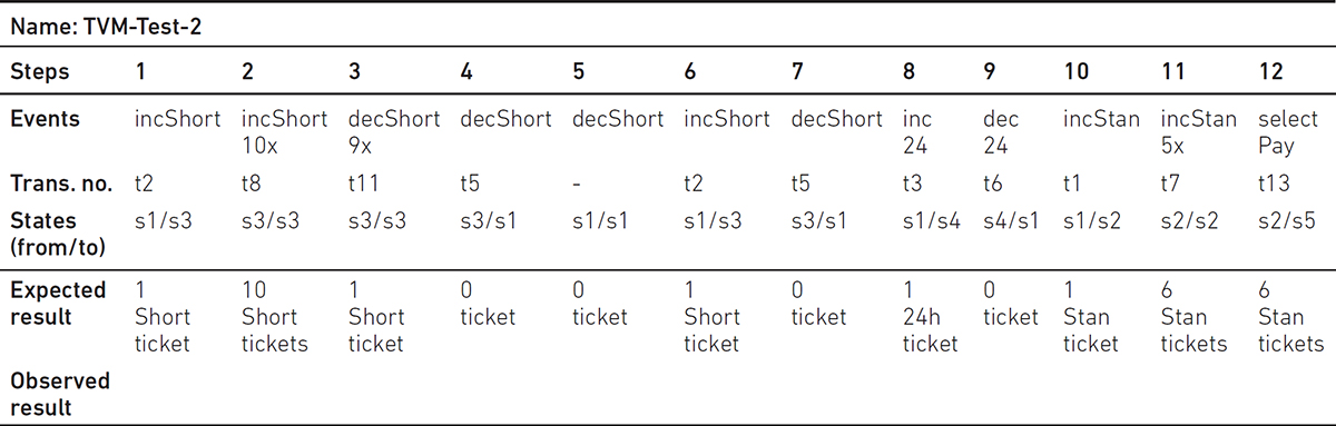
Table 6.11c State transition tests for the TVM-Test-3
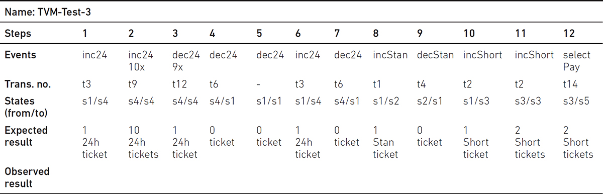
Table 6.11d State transition tests for the TVM-Test-4
Name: TVM-Test-4 |
||
Steps |
1 |
2 |
Events |
incStan |
selectPay |
Trans. no. |
t1 |
t13 |
States (from/to) |
s1/s2 |
s2/s5 |
Expected result |
1 Stan ticket |
1 Stan ticket |
Observed result |
|
|
Table 6.11e State transition tests for the TVM-Test-5
Name: TVM-Test-5 |
||
Steps |
1 |
2 |
Events |
incShort |
selectPay |
Trans. no. |
t2 |
t14 |
States (from/to) |
s1/s3 |
s3/s5 |
Expected result |
1 Short ticket |
1 Short ticket |
Observed result |
|
|
Table 6.11f State transition tests for the TVM-Test-6
Name: TVM-Test-6 |
||
Steps |
1 |
2 |
Events |
inc24 |
selectPay |
Trans. no. |
t3 |
t15 |
States (from/to) |
s1/s4 |
s4/s5 |
Expected result |
1 24h ticket |
1 24h ticket |
Observed result |
|
|
This example will be extended in the Gherkin-based test design chapter (Chapter 12) by paying for the tickets. In that case, STT and EP and BVA shall also be applied together.
METHOD EVALUATION
In this section we evaluate the state transition test design technique from various perspectives.
Applicability
The state transition testing technique can be applied when the system is defined in terms of a finite number of states and the transitions between the states are triggered by the rules of the system. Practically, the technique is usable for real applications involving states and transitions. This method is especially good for end-to-end testing of large systems, testing embedded systems, web applications, compilers, telecommunication protocols and so on.
Types of defects
The technique can detect integration and system errors even in large systems. Typical defects include incorrect or unsupported transitions, unreachable or non-existent states, omissions (there is no information about what the automaton should do in a certain situation) and inconsistent model descriptions. State transition testing can reveal some predicate errors as well.
Advantages and shortcomings of the method
The advantages of the state transition testing method are:
• State transition diagrams can be created for many applications, hence this testing technique is widely applicable.
• Other test design methods can be involved in state transition testing.
• There exist numerous test selection criteria, from linear up to exponential.
• State machines can be easily used for automated test design (such as model-based testing).
• In large systems, the models can be built up in a hierarchical manner.
The limitations and shortcomings of the method are:
• Constructing the state model is not always easy. If the graph is complex, then even a professional tester may make mistakes.
• The tests have to be carefully validated, which is not always simple.
• At the time of writing, there is no tool for automating test case generation based on all of the featured test selection criteria.
• Achieving high switch coverage levels implies almost always combinatorial explosion in the number of test cases.
• Sometimes it is difficult to include negative tests. The tester shall consider these tests additionally.
• Complex event-driven systems, where various data structures have to be handled concurrently (stack, FIFO, i.e. first in, first out, etc.), are hard to describe by FSMs because of the state space explosion. In such cases other modes are suggested, for example pushdown automaton.
THEORETICAL BACKGROUND
A state machine is a mathematical model of computation. The roles of state machines in software testing are: (1) before starting the actual implementation, an executable state machine may simulate the model with event sequences as test cases, (2) supports testing against the specification and (3) supports automatic test generation (there should be an explicit mapping between the state machine elements and the elements of the implementation, e.g. classes, objects, attributes, etc.).
The behaviour of discrete systems can be described by different models. Labelled or unlabelled transition systems are used to describe dynamic processes with configurations representing states and transitions prescribing how to go from state to state. Transition systems are mathematically equivalent to abstract rewriting systems or with directed graphs. Finite-state machines differ from them in several ways, namely, FSMs have a finite set of states and transitions, and have start nodes and so on. FSMs have less computational power than Turing machines or pushdown automatons since their memories are limited by their finite number of states. State machines are used to give an abstract description of the system’s behaviour. This behaviour is analysed and represented as a series of events that can occur in one or more possible states. State diagrams are used to graphically represent those (finite-state) machines. Many forms of state diagrams exist, which are all slightly different.
Statecharts refer to Harel’s notation described in Harel (1987), which was proposed as a significant notational extension over traditional finite-state machines. Statecharts have been incorporated in the UML by introducing the concept of hierarchically nested states (logically connected subgraphs can cluster into a new super-state) and orthogonal regions (orthogonality means compatibility and independency in the given context). With this hierarchical clusterisation, the state transition testing becomes possible even for large systems. UML state machines have the characteristics of both Mealy and Moore machines.
Specification and Description Language (SDL) state machines from the ITU (International Telecommunication Union) include graphical symbols to describe the actions in the transitions (timers, sending, receiving messages, etc.). SDL combines together abstract data types, an action language and an executing semantic to make the machine executable.
While using an FSM for embedded system design, the inputs and outputs are Boolean data types, and the functions represent Boolean functions with Boolean operations. This model is enough to describe control systems without involving input or output data. When data is to be dealt with, EFSM is needed.
The applicability of state diagrams in testing was observed in the 1970s. One of the first and the most cited papers is the work of Chow (1978), who proposed a method of testing the correctness of control structures that can be modelled by a finite-state machine. Test results derived from the design are evaluated against the specification. No ‘executable’ prototype was required. Clearly, his testing method was an early test-first method. You can read more on this topic in Chapter 11.
KEY TAKEAWAYS
• Stateful systems are able to ‘memorise’ the preceding user interactions or events; the remembered information is the state of the system. They exhibit different behaviours in different states. State transition diagrams are used to describe the behaviour of stateful systems. State transition testing is used for testing them.
• There are several test selection criteria available for state transition testing by which the test design can often be automated.
• For real specifications, various test design methods (like EP, BVA and STT) can be applied in combination.
• To catch data-flow defects among transitions and states the all-transition-state and all-transition–transition criteria were suggested.
EXERCISES
E6.1 Construct test paths applying the all-transition–transition criterion for ‘TVM ticket selection’ (see TVM example earlier in the chapter and Figure 6.7).
E6.2 Ordering water from an online shop. The types of water can be still or sparkling. We can buy bottles of one type only. If nothing is selected, then the quantity of either of them can be increased. After one has been selected, only one of the water types with a non-zero amount can be increased or decreased by one. The maximum number of bottles to be ordered is five. If the selected number of bottles is greater than 0, then the buying process can start. The output is the type and number of the selected bottles.
Model the buying process for this example with a state transition graph and design tests for the following test selection criteria:
1. All-transition criterion.
2. All-2-transitions criterion.
3. All-transition-state criterion.