9 COMBINATIVE AND COMBINATORIAL TESTING

Combinatorial testing aims to determine data combinations to be tested. In a complex testing environment, this testing technique has practically two main application areas: (1) testing combinations of configuration parameter values and (2) testing combinations of input parameter values. Multidimensional EP and BVA testing is a special case in the latter.

In combinative testing, the number of reliable tests can be described by a linear function of the maximal number of parameter values or by the number of parameters. This is especially useful when a large number of parameter combinations is given.

Let’s look at an example. Given n parameters, when each of them can have m_i different values (i ϵ {1, 2,…,n}), the question is how to choose a reliable test set among the parameter values. Unfortunately, testing all of the possible combinations m₁ × m₂ × … × m_n may result in a large number of test cases that is infeasible and inefficient – exhaustive testing of complex computer software is still impossible.

Fortunately, thorough investigations show that a considerable percentage of software faults are triggered by a single parameter, while most of the faults arise from the interaction of two or just a few parameters (see Kuhn et al., 2008). Concentrating on those combinations, testing may become more effective in practice. Kuhn determined that up to 97 per cent of software failures can be detected by only two variables interacting and practically 100 per cent of software failures are detected by at most six variables in combination. This means that testing every combination up to six variables can be considered practically as good as exhaustive testing.

Figure 9.1 Fault detection at interaction strength according to Kuhn et al. (2008). The region shows the most probable fault detection rate in various interaction levels

To deal with the combination set, the main problems are:

Before we discuss the various selection techniques let’s consider the extreme cases. When the test suite is created randomly, the sampling is based on some input distribution (often uniform distribution). Not underestimating the power of random choice, do you really want to design your test cases randomly?

On the other hand, when every combination of each parameter value is used, the number of test cases can be large; in our example above it is 4 × 3 × 2 × 4 = 96. Of course, in general, this is not feasible.

Real combinatorial testing is expensive as it requires an over-linear number of test cases. However, for non-safety critical programs, this is usually not necessary. Let’s assume a large program with 5000 test cases. Let’s also assume that we would like to extend the test by combinatorial testing, but only for four per cent of the tests. This means that 5000 × 0.04 = 200 test cases should be extended. Combining all test data pairs results in 200 × 200 = 40,000 test cases (all pairwise combinations), that is, the total number of test cases will be 40,000 + 5000 × 0.96 = 44,800 at worst case. This means that the number of test cases has increased by 796 per cent.

For normal projects this growth is impossible. Let’s assume that we have a technique by which the number of reliable tests is just doubled. Considering the same example, the total number of test cases will be 5200 at worst case, where the growth is only four per cent. This is usually manageable, especially if we also detect tricky bugs, the fixing of which would be more expensive than the additional testing cost. Therefore, linear and yet reliable techniques are preferable.

COMBINATIVE TECHNIQUES

Combinative test design techniques are easy to generate, with the number of test cases depending linearly on the maximal number of parameter values.

Diff-pair testing

The rationale behind the combinative technique introduced in this book is to ensure that for a single variable each computation is calculated in more than one context. The basic variant of the presented combinative testing is called diff-pair testing. Informally, it requires that each value p of any parameter P be tested with at least two different values q and r for any other parameters. For example, if the parameter P has two possible values, let us say x and y, and there are two more parameters Q and R with values: Q: (1, 2) and R: (Y, N), then we have to test the value pairs (x, 1), (x, 2), (x, Y), (x, N). Thus, the test suite required for testing parameter P contains the data combinations {(x, 1, Y), (x, 2, N)} or {(x, 1, N), (x, 2, Y)}. Similarly, for y, we test {(y, 1, Y), (y, 2, N)} or {(y, 1, N), (y, 2, Y)}.

We test the values of the other parameters R and Q similarly. More formally, diff-pair testing requires the testing of each parameter pair (P, Q) in such a way that there should be at least two test data pairs (pi, qj) and (pi, qk) present in the test suite for each pi ϵ P, qi, qk ϵ Q, where qj ≠ qk.

Example diff-pair

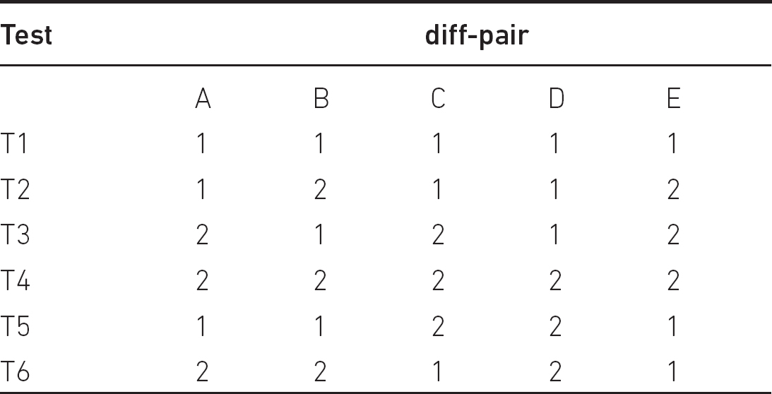
Suppose that we have five parameters (A, B, C, D, E) and all of them have two possible values, 1 and 2. Then the test sequences shown in Table 9.1 satisfy the criteria of diff-pair.

For example, let’s see the third parameter C:

Consider now the last parameter E:

We leave the remaining three parameters to the reader.

Diff-pair-N testing

We can extend diff-pair testing in such a way that for a pair of test data not only one but N parameter values are different.

Table 9.1 Diff-pair example for five parameters having two values each

The technique requires the testing of each parameter value p ϵ P at least twice in the following way: there must always be at least two tests such that whenever both tests contain data p, then for all other arbitrary N parameters their data values differ, that is if

T1 = (p, q1, q2,…,qN,…) and

T2 = (p, q1’, q2’,…,qN’,…)

then q1 ≠ q1’, q2 ≠ q2’,…,qN ≠ qN’.

Diff-pair testing is actually diff-pair-1 testing. Experience shows that in most of the cases the value N = 1 is strong enough.

Example diff-pair-4

Let the five parameters (A, B, C, D, E) with values 1 and 2 be given again. Then the test sequences in Table 9.2 satisfy the criteria of diff-pair-4.

Example diff-pair-3

The diff-pair-3 test set for the ‘Configuration Testing’ example can be seen in Table 9.3.

Then, the parameter value

Table 9.2 Diff-pair-4 example for five parameters having two values each

Table 9.3 Diff-pair-3 tests for the ‘Configuration Testing’ example

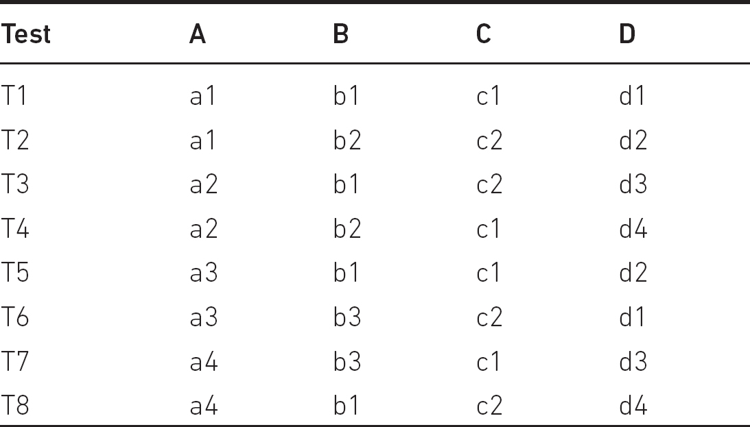
Note that for this example the same number of test cases are required for diff-pair-1 (diff-pair) testing.

Consider the diff-pair technique. We prove that the number of test cases remains linear. Assume that we have the parameters A, B, C,…,Z with values a1, a2,…,an, b1, b2,…,bn, …z1, z2,…,zn. Let’s generate 2n test cases in the following way.

It is easy to see that each data aj appears in two test cases for all j ϵ {1,…,n}. For example, a1 appears in T1 and T(n+1) but all the other parameter values are different in those tests. Similar reasoning can be given for other parameter values, since in the first n tests the values have the same indices in a test, while in the second n test cases the indices are permutations.

We can see that in this case, assuming that n is not less than the number of parameters, these test cases also satisfy diff-pair-n. If the number of test cases can be the same for diff-pair-k and diff-pair-n technique, we have to satisfy the stronger technique. This was the case in our ‘Configuration Testing’ example. In general, if diff-pair-k testing requires a minimum of K test cases and with K test cases we can cover diff-pair-m as well (m > k), then diff-pair-k testing satisfies diff-pair-m testing.

COMBINATORIAL TECHNIQUES

The aim of combinatorial testing is to produce high-quality tests at a relatively low cost even if the number of the possible data combinations are over linear.

Base choice

This technique starts with identifying the base test case. The choice depends on any test object-related criterion: most risky, most likely values and so on. Then, the other test cases are created by varying the base test case by one parameter value at a time in all possible ways, while keeping the other values fixed (see Table 9.4).

Clearly, the technique satisfies the 1-way coverage. The number of test cases in our example is 1 + (4 – 1) + (3 – 1) + (2 – 1) + (4 – 1) = 10. In general, considering n different parameters having m different values, the number of test cases is 1 + n x (m − 1).

Table 9.4 ‘Configuration Testing’ example: base choice

N-way testing

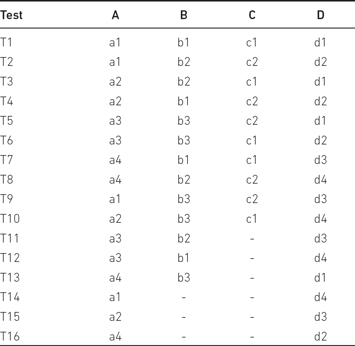
This technique takes N-way combinations of all the parameter values, eliminates the combinations that are unlikely or impossible, and uses the realistic combinations for testing. Though the method can be automated, only 2-way (pairwise) or 3-way testing is realistic in practice. At most those cases are computationally tractable and effective. In our ‘Configuration Testing’ example the all-pairs table is shown in Table 9.5.

In the table ‘-’ denotes the ‘don’t care’ symbol. Please check that all data value pairs can be found in a test case, for example a2–d4 pair is in T10.

The convention for describing the variables and values (called configurations or signatures) in combinatorial testing is v₁^k1v₂^k2…, where v_i are the size of the variable sets and k_i are the number of their occurrences. Our ‘Configuration Testing’ example has the signature 2×3×4². To get an insight into the reduction rate of N-wise combinatorial techniques, the examples in Table 9.6 show the number of tests for various configurations.

The number of test cases including all N-way combinations depends on:

Table 9.5 All-pairs tests for the ‘Configuration Testing’ example

To be more precise, the number of N-way tests is proportional to v^N×log(n) for n parameters with v values each. Hence, the method is reasonable even for larger parameter spaces (i.e. v ≤ 10 and N = 2,3). For example, if there are 20 variables with 10 different values each, then using pairwise testing, 180 test cases are sufficient. Exhaustive testing would need 10²⁰ tests. This logarithmic growth means that if a project uses combinatorial testing for a system having (let’s say) 30 parameters and applies a few hundred tests, then the larger system with 40 parameters (after 5 years in the project life cycle) may only require a few dozen more tests. Hence, it is scalable.

Note that although pure random choice covers a high percentage of N-way combinations, increasing the coverage level requires significantly more and more tests. For example, the configuration 4¹⁰ (10 parameters with four values each) can be covered with 151 tests by applying 3-way testing. However, pure random generation needs over 900 tests to provide full coverage.

There are supporting tools for N-way test generation. Moreover, these tools allow the inclusion of certain important configurations, relevant interactions, and take into account constraints, or impossible combinations.

Table 9.6 Comparison of some combinatorial methods

Orthogonal arrays

Orthogonal array (OA) testing is a systematic, statistical method for constructing parameter value combinations. It is used when the parameter space is large, but the number of possible values per parameter is small. It is especially effective in finding logic errors in complex software systems (e.g. in telecommunications).

An orthogonal array OA(N, t, k, v, λ) is an N x k array with the following property: in every N x t subarray, each t-tuple occurs exactly λ times. We refer to t as the strength of the coverage of interactions, k as the number of parameters or components (degree), and v as the number of possible values (levels) for each parameter or component (see Kuhn et al., 2008). The property for the t-tuples shows a kind of ‘orthogonality’, where the method name comes from.

A test suite based on an orthogonal array of strength t = 2 satisfies the criterion of pairwise testing, that is, for every pair of factors all possible pairs of the test values are exercised. The clear advantage of the test suites based on OAs is the size of the test set. For example, in the case of t = 2, v = 2, k = 11 the array has N = 12 columns (λ = 3); in the case of v = 2, k = 15 the array has N = 16 columns (λ = 4); in the case of v = 3, k = 13 the array has N = 27 columns (λ = 3) and so on.

Practical considerations

For mixed OAs, where there are various factors and levels, the test generation is still useful. The system 2⁹×4² (nine factors with level = 2 and two factors with level 4) has 16 runs (λ = 4). For the pairwise cases (t = 2) some descriptions use the notation L_Runs(Levels^Factors) for OAs. Here

The basic process of using OA to select balanced pairwise subsets is:

Regarding the last two steps, note that you do not have to create the OA. You have to figure out the proper size of the array (various websites¹ maintain comprehensive OA catalogs of orthogonal arrays) then harmonise the test problem with the array.

OA does not guarantee 100 per cent (pairwise) test coverage; it can only ensure a balanced one. Scripts generated through OA have to be manually validated, and additional test cases have to be added to ensure better test coverage.

However, there are limitations for orthogonal test design: (1) such OA may not exist, (2) for a given OA the test cases (designed based on the requirements basis) may contain invalid pairs of tests. For example, an orthogonal array with strength = 2 and structure 2⁴ × 3¹ does not exist. In such cases, a suitable OA is modified to fit the need.

Covering arrays

Fortunately, there is a generalisation for OAs in the sense that the test suite should cover all valid pairs of test values with as-few-as-possible test cases (Sloane, 1993) (supposing that no fault involves more than two factors jointly). A fixed-value covering array CA(N, v^k, t) is an N x k matrix of entries from the set {0, 1,…, (v-1)} such that each set of t-columns contains every possible t-tuple of entries at least once. Similarly, a mixed-value covering array CA(N, v₁^k1 v₂^k2 … v_n^kn, t) extends the fixed value, where k = k1 + k2 + … + kn. In other words, k_i columns have v_i distinct values. All orthogonal arrays are covering arrays but not vice versa.

Table 9.7 Covering array for 2¹ × 3¹ × 4²

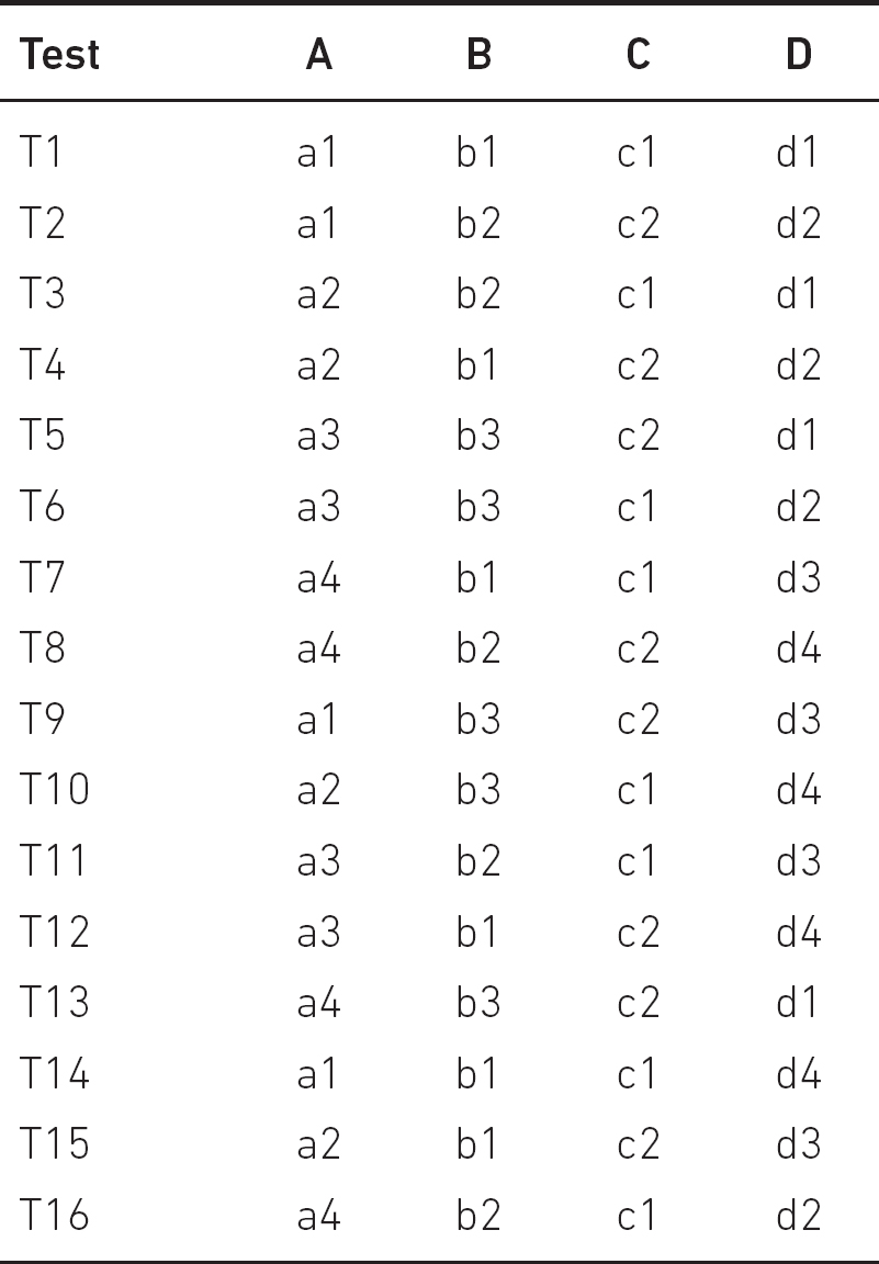
In our ‘Configuration Testing’ example, we have two factors (parameters) with four options, the others have just three and two. The covering array for 2¹ × 3¹ × 4² is shown in Table 9.7.

In the table, in any two columns, the pairs appear a maximum of two times. Observe that the (a_i, d_j) pairs appear exactly once.

Note that orthogonal arrays are likely to produce more test cases than covering arrays.

COMPARISON OF THE TECHNIQUES

There are different types of faults, such as logic, computational, interface, data handling and so on (see IEEE 1044, 2009). Basically, there are two main types of programming errors (Howden, 1976): (1) computation error and (2) control-flow error. A program is said to cause a computation error if a specific input follows a correct path, but the output is incorrect due to faults in some computations along the path. A control-flow error occurs when a specific input traverses a wrong path because of faults in the control flows of the program. For simplicity, it is assumed that the control-flow error involves the missing case errors as well (when some control in the code is missing). In this section, we compare the previously defined combinatorial techniques and investigate their reliability. We provide two examples, one related to computation, the other one to control-flow errors.

Example: testing computation errors

Assume that we have one of the following code excerpts (we neglect function and variable declarations):

// Correct implementation (excerpt)

 1. if price == 0 then return(0);

 2. if VIP == true then

 3.       price = price * 0.9;

 4. if delivery == local then

 5.       price = price * 1.02;

 6. else if delivery == city then

 7.       price = price * 1.05;

 8. else price = price * 1.08;

 9. if packaging == basic then

10.       price = price + 1;

11. else if packaging == safety then

12.       price = price + 4;

13. else if packaging == exclusive then

14.       price = price + 5;

15. else price = price + 9;

// Implementation with three bugs

 1. if price == 0 then return(0);

 2. if VIP then

 3.       price = price * 0.9;

 4. if delivery == local then

 5.       price = price * 1.02;

 6. else if delivery == city then

 7.       price = price * 1.08; //BUG HERE

 8. else price = price * 1.08;

 9. if packaging == basic then

10.       price = price + 1;

11. else if packaging == safety then

12.       price = price + 1;//BUG HERE

13. else if packaging == exclusive then

14.       price = price + 5;

15. else price = price + 8;//BUG HERE

Of course, the tester knows nothing about the implementation. After analysing the specification, the clever tester asks for the average purchase amount (needed for the tests). The sales department answers that it is around EUR 70–100. Since the project is ‘extremely agile’, the tester does not want to write more than 10 tests. You may ask, how many test cases would result in the all-pairs technique? Table 9.8 shows a possible set of tests for the correct implementation (rounding is to one euro cent).

We have only 12 test cases, while exhaustive testing would require 24. Note that product price is not a parameter here as it is not mentioned explicitly in the specification. Hence, we could have selected the same price for each test.

Let’s consider the base choice method with the basis parameter set (VIP, Basic, Town) (Table 9.9).

Based on Tables 9.8 and 9.9 you can observe that Test2 = T3, Test3 = T1, Test4 = T2, Test5 = T6, Test6 = T8, Test7 = T12. Now the test suite reveals two out of the three bugs. Let’s suppose that the developer corrects line 7 and line 12 in the buggy code and reruns the previous test suite against the corrected code. Then all of the tests pass. To summarise, this method has a shortcoming: the fault in line 15 has not been revealed.

Table 9.8 Tests for the ‘Packaging and delivery service’ example

Table 9.9 Base choice tests for the ‘Packaging and delivery service’ example

Finally, let’s consider the diff-pair technique (see Table 9.10).

First, we check the fulfilment of the diff-pair criteria.

Table 9.10 Diff-pair tests for the ‘Packaging and delivery service’ example

After running the test set against the faulty code three bugs can be found.

Hence, this eight-test set is reliable. This shows the power of the method. If the tester chooses another diff-pair test set, similar results can be obtained.

Observe that the erroneous code contains only the typos 5 to 8 (line 7) and 4 to 1 (line 12) and 9 to 8 (line 15), therefore the competent programmer hypothesis is not violated. Clearly, the pairwise test set gives a similar result with 12 tests.

Example: Testing control-flow errors

This next example demonstrates the usage of combinatorial test design techniques together with other traditional design techniques. We concentrate on control-flow errors.

We have three equivalence partitions concerning the price reduction: 0-99.9, 100-199.9, 200 and above. According to the test selection criterion discussed in Chapter 5, we can apply the following boundary values for testing: 0, 99.9, 100, 199.9, 200, 10,000. We have three possible customer statuses: non-VIP, normal VIP and premium VIP customer (exclusively). The prepaid status can be YES or NO. Altogether we have 6 × 3 × 2 = 36 possible data combinations.

We do not consider any unstructured, un-refactored code (however, it exists in practice).

Suppose that we have the following Python code:

# Correct implementation

def webshop(price, vip, prepay):

  reduction = 0

  if price >= 200:

    reduction = 8

  if price >= 100 and price < 200:

    reduction = 4

  if vip == 'normal':

    reduction = reduction + 1

  if vip == 'premium':

    reduction = reduction + 3

  if prepay == True:

    reduction = reduction + 3

  return(price*(100-reduction)/100)

# Buggy implementation

def webshop(price, vip, prepay):

  reduction = 0

  if price >= 200:

    reduction = 8

  if price >= 100 and price <= 200:#BUG HERE

    reduction = 4

  if vip == 'normal':

    reduction = reduction + 1

  if vip == 'premium':

    reduction = reduction + 3

  if prepay == True: #BUG HERE

    reduction = reduction + 3

  return(price*(100-reduction)/100)

The number of test cases for pairwise testing is 18, and the possible test cases against the faulty implementation are in Table 9.11.

When the tester chooses some EP and BVA tests, for example T1, T3, T5, T7, T11, and, for the price EUR 200, any one of T9, T10 or T17, then they will find the bug.

Suppose that the bug is corrected (shaded line in the faulty code) and the tests changed (see Table 9.12).

Now, the EP and BVA test suite TS = {T1, T3, T5, T7, T10, T11} does not reveal the remaining control-flow bug.

Let’s construct a test suite satisfying the diff-pair criterion. Consider the test suite in Table 9.13.

Table 9.11 Pairwise tests for the ‘Online Shop’ example

Table 9.12 Changed tests for the ‘Online Shop’ example

We check the fulfilment of the diff-pair criterion:

Observe that the test cases Test9 and Test10 detect the bug, hence, our method is reliable.

Table 9.13 Diff-pair tests for the ‘Online shop’ example

Clearly, there are bugs for which neither the diff-pair-N nor even the pairwise methods are reliable. However, even in these cases, in applying the diff-pair technique, the probability of revealing the bug is considerable.

CLASSIFICATION TREES

A classification tree (CT) is a graphical technique by which various combinations of conditions can be tested. The technique allows combining EP and BVA with combinatorial methods. The process of constructing CTs consists of the following steps:

Each test object can be typified by a set of classifications (input parameters, environment states, preconditions, etc.). Each classification can then have any number of disjoint classes. These classes describe the parameter space. The class selection mechanism is basically an equivalence partitioning (forming abstract test cases). Then, BVA is applied to the classes producing the concrete test cases. This structuring results in the classification tree.

If the classification tree has been created, the next task is to specify suitable test cases. A test case specification comes from the combination of classes. The minimum number of test cases is usually (but not necessarily) the maximal number of classes in the classification. The maximal number of test cases is the Cartesian product of all classes of all classifications.

Figure 9.2 Classification tree for the ticket selection process. We used BVA for the Amount class data. The highlighted tests are the negative tests

There are commercial tools² for supporting CT drawings with various test case selection mechanisms incorporated.

A ticket selection process (similar to our TVM) can be modelled with the classification tree shown in Figure 9.2.

This technique can be used at any level of testing. We suggest you start with small tables (at a high level). If your tree becomes too large, break it down, referring to a higher-level tree.

Probably the greatest benefit of CTs is when there is a continuous need for maintenance. In these cases its graphical approach provides an easy-to-follow overview.

TVM EXAMPLE

Here we design test cases for the following part of the TVM.

As the risks are not very high, we apply diff-pair testing. Let’s consider item 6 in Chapter 3, Table 3.2:

Though these features (timeout, delete) are different, they can be used interchangeably. If reset does not work, we can wait for timeout. If timeout does not work when a guest leaves the TVM, the next guest can use the reset function. Therefore, we consider an aggregate parameter Delete with three values: No, Reset, Timeout.

We start from the test cases of TVM in Chapter 5. We had seven test cases. We extend the test cases by the values of Delete. During the (later) actual test execution, we first insert the coins, then press reset or wait for the timeout. The test cases are shown in Table 9.14.

Table 9.14 Test design for the TVM example

We can see that the number of test cases has doubled, and we design inputs Reset and Timeout for each EP, maximising the diversity as much as possible. For the test cases with Reset or Delete, we only validate whether we can go to the initial screen in all circumstances. Therefore, in these test cases, it is unnecessary to check RAP and acceptable banknotes. That’s why we used strikethrough characters.

METHOD EVALUATION

Combinatorial testing provides a means to identify an appropriate subset of data combinations, where the data combinations come from combinatorial combinations. The aim is to achieve a predetermined level of coverage.

Applicability

Combinatorial testing is used extensively in:

Configuration testing is probably the most commonly used application of combinatorial methods in software testing.

We suggest using combinative testing with a trade-off for higher risks and manageable test effort. The optimum costs described in Chapter 3 can be often reached by applying diff-pair testing, as we can unfold bugs undetectable by other non-combinatorial techniques at low additional testing effort.

Types of defects

The most common type of defects related to combinatorial testing arises from the combined values of several parameters.

Advantages and shortcomings of the method

Combinatorial testing reduces the overall number of test cases compared to exhaustive testing. Combinative testing further reduces the number of combinatorial test cases. They detect:

Combinative and combinatorial testing can be automated in part, that is the input combinations can be generated. The technique can be applied at any level of testing. Classification trees raise the visibility of test cases and improve maintainability.

The key limitation of combinatorial test design is the testing cost, due to its non-linearity. For high risk software generating N-way tests, the oracle problem is challenging. Moreover, efficient N-way testing requires that:

In most cases, fixed-level orthogonal arrays (same number of values for each parameter) do not exactly match to the current test problem. For mixed level orthogonal arrays there are many options to choose, hence, finding the optimal one can be difficult.

THEORETICAL BACKGROUND

Combinatorial testing is an application of the mathematical theory called combinatorial design. It concerns the arrangements of a finite set of elements into various patterns (subsets, words, arrays, etc.) according to specified rules. Generating the optimised list of such combinations for specific input is an NP-hard problem (they are at least as hard as the hardest problems in NP). With the increase of the input parameters, there is an exponential increase in the computational time as well as in the degree of the problem complexity. Hence, there is a need for efficient and intelligent strategies for generation.

There exist three different types of methods for constructing combinatorial test suites:

The first group of methods do not result in accurate results on general inputs; however, they are very quick. The second group has been found to be relatively efficient regarding running time and accuracy. The heuristic search provides even more accuracy at the expense of execution time. The first and widely cited heuristic approach was implemented in the Automatic Efficient Test Generator (AETG) System (Cohen et al., 1997).

For software testing, Mandl was the first to propose pairwise combinatorial coverage to test the Ada compiler in 1985 (Mandl, 1985). He generated appropriate test sets as well. There is a comprehensive survey of this topic by Nie and Leung (2011). Another good review article has been written by Czerwonka (2008).

The classification tree method was developed by Grochtmann and Grimm (1993) partly using and improving ideas from the category-partition method defined by Ostrand and Balcer (1988).

In many systems, the input is a permutation of some event set. One can define a sequence covering array in such a way that the test suite ensures testing of all N-way sequences of events. Normal covering arrays are unusable for generating N-way sequences since they are designed to cover combinations in any order. However, in a sequence covering array, every N-way arrangement of variables, v₁, v₂,…,v_N, the regular expression .*v₁.*v₂...*v_N.* should match at least one row in the array.

Sequence covering arrays are developed to solve interoperability testing problems. For more details see Kuhn et al. (2012).

KEY TAKEAWAYS

EXERCISES

E9.1 Consider the specification of E5.1 (Payment). Design test cases by applying the diff-pair testing technique.

E9.2 You want to test your favourite word processor. You are interested in the following attributes in combination:

Construct test cases for pairwise testing.

1 https://www.york.ac.uk/depts/maths/tables/orthogonal.htm
http://neilsloane.com/doc/cent4.html

2 https://www.razorcat.com/en/product-cte.html
https://www.assystem-germany.com/en/products/testona/classification-tree-method/