![]()
Integration with Python
This chapter shows you how to use Python in Azure Machine Learning (Azure ML). Using simple examples, you will learn how to integrate Python as part of an Azure ML experiment. This enables you to tap into the powerful capabilities offered by various Python libraries, such as NumPy, SciPy, pandas, scikit-learn, and many more, directly in an Azure ML experiment.
Python is an elegant and powerful interpreted programming language. Both R and Python rank amongst the top programming language of choice for data scientists and developers. Python empowers data scientists and developers to use it in early experimentation and to have confidence in deploying it into production environments. Many large organizations, including YouTube, Industrial Light & Magic, IronPort, HomeGain, and Eve Online, have used Python successfully in production (www.python.org/about/quotes/).
Since the invention of Python by Guido van Rossum at Centrum Wiskunde & Informatica (CWI) in the late 1980s, many powerful Python libraries for performing data analysis have been made available, including the following:
- NumPy (Numerical Python): Provides fast and efficient multidimensional array operations, a rich set of linear algebra methods, and random number generators.
- pandas: Provides powerful data processing capabilities (reshaping, slicing and dicing, aggregations, filtering) for structured data sets.
- SciPy: Provides a rich set of mathematical and utility functions. SciPy is organized as subpackages, and each subpackage is used for data analysis. The capabilities offered by the subpackages range from fast Fourier transforms and interpolation methods to a large collection of statistical distributions and functions.
- scikit-learn: Provides an extensive set of machine learning capabilities including classification, regression, cluster, dimensionality reduction, model selection, and data preprocessing.
- matplotlib: Enables users to easily generate charts and visualizations.
Besides these general-purpose Python libraries, there are many domain-specific Python libraries available for applications ranging from computational biology and bioinformatics to astronomy. For example, BioPython is used by data scientists in the bioinformatics community for processing biological sequence files as well as working and visualizing phylogenetic trees. As of May 2015, the Python Package Index (https://pypi.python.org/pypi), a repository for Python libraries, contained 59,717 Python packages.
If you are a Python expert, this chapter enables you to quickly understand how you can leverage familiar tools and integrate the Python scripts into an Azure ML experiment. If you are new to Python, this chapter helps you gain the basics of using Python for data analysis and pre-processing, and sets you up for a successful Python learning journey. This chapter is not meant to be a replacement of the many excellent Python online resources and books; in fact, this chapter offers references to useful Python online resources that you can tap into.
Let’s get started with understanding how Python can be used with Azure ML.
Python provides an interactive command-line shell that enables you to work with Python code. In addition, the IPython Notebook provides a rich, interactive browser-based environment for executing Python code and visualizing the results. In this chapter, you will run the Python code in an IPython notebook.
To get started, download Anaconda from http://continuum.io/downloads. Anaconda provides a free Python distribution that you can use. In this chapter, we will focus on running IPython on Windows. In addition, the Anaconda installation installs the IPython notebook. After you have installed Anaconda, you can perform the following steps to create the IPython notebook.
- Press the Windows button, and type IPython. Figure 5-1 shows the search results.

Figure 5-1. Searching for IPython Notebook
- Start the IPython server by clicking the IPython (Py 2.7) Notebook.
- Once the IPython server is started, it automatically navigates to .
- Once you are on the IPython home page, you can create a new Python notebook by clicking New, and choosing Python 2 notebook. Figure 5-2 shows how to create the notebook.

Figure 5-2. Creating a Python 2 notebook
- After the notebook has been created, you can navigate to the new notebook.
- Type print "Hello World" and click the Run button. Figure 5-3 shows the Hello World example.

Figure 5-3. Hello World Example
You can use IPython notebook to develop your Python script and test it before integrating it with Azure ML. To use Azure ML with your Python environment, you will need to install the AzureML Python module. To do this, follow these steps.
- Press the Windows button, and type Command Prompt. Figure 5-4 shows the search results.

Figure 5-4. Using the command prompt
- Select Command Prompt, and navigate to the folder where you have installed Python. For this exercise, we will assume that Python is installed in C:Python34.
However, depending on your installation, you might find Python installed in the default installation folder, C:UserslocaluserAppDataLocalContinuumAnaconda.
- Set the path using the command prompt:
path=%path%;c:python34scripts - After you have set the path successfully, you can use the pip command to install the AzureML module, as follows:
pip install azureml
After you have installed the azureml module successfully, you can use it in an IPython notebook. Figure 5-5 shows the azureml module installed successfully.
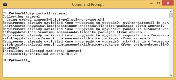
Figure 5-5. Installing the azureml module
In the next section, you will learn how to use the IPython notebook to access the data used in an Azure ML experiment.
![]() Note Learn more about Python at www.python.org/ and design philosophies in the “Zen of Python” at www.python.org/dev/peps/pep-0020/.
Note Learn more about Python at www.python.org/ and design philosophies in the “Zen of Python” at www.python.org/dev/peps/pep-0020/.
Using Python in Azure ML Experiments
Let’s get started on using IPython notebook to work with the experiments in ML Studio. But first, let’s use one of the sample experiments from the gallery.
- In your web browser, navigate to the following URL: http://gallery.azureml.net/browse/?tags=["demandestimation"].
You can also search for the experiment in the gallery by using the keywords demand estimation.
Figure 5-6 shows the sample experiment for demand estimation. This experiment shows how to build a regression model for bike rental demand.

Figure 5-6. Getting to the sample experiment called Regression: Demand estimation
- Click the Regression: Demand estimation experiment. Figure 5-7 shows the experiment and the data used in the experiment.

Figure 5-7. The Regression: Demand estimation experiment
- Click Open in Studio to view the experiment in ML Studio (see Figure 5-8).

Figure 5-8. Running the regression experiment
 Note If you have an Azure subscription, you can create a Machine Learning workspace using https://manage.windowsazure.com.
After you open the experiment in ML Studio, you can copy the experiment into the workspace you have created. To view the experiment, you can use the 8-hour guest access option by clicking GUEST ACCESS when entering ML Studio.
If you are using GUEST ACCESS, you will not be able to run the experiment, and you will have to sign in using a valid Microsoft account.
- After you open the experiment in ML Studio, run the experiment by clicking the Run button at the bottom of the ML Studio.
- Suppose in this experiment you want to make use of Python for pre-processing the input data before using it as inputs to the rest of the ML modules. To do this, right-click the node for the Bike Rental UCI Dataset- Copy.
- Click Generate Data Access Code, as shown in Figure 5-9.

Figure 5-9. Generating data access code
- This will generate the data access code in Python (shown in Figure 5-10). You can paste the data access code into a new IPython notebook.
The Python code contains the information needed to access the specific dataset and the authorization_token.

Figure 5-10. Data Access Code
- Copy and paste the Python code into the IPython notebook, as shown in Figure 5-11.

Figure 5-11. Using IPython notebook to access the dataset
- In the Python code snippet that you have pasted, you can see that you are accessing the dataset in the workspace by name, where you specified the name of the dataset as Bike Rental UCI dataset – Copy(2).
After you have the data, you converted it into a pandas dataframe using the ds.to_dataframe() function.
Note You can find out more about the internals of the AzureML Python library in the GitHub repository at https://github.com/Azure/Azure-MachineLearning-ClientLibrary-Python. - In the next IPython notebook cell, type frame, and click Run Cell (as shown in Figure 5-12).

Figure 5-12. Running the data access code
- After you run the selected cell, you will see the data contained within the pandas dataframe, as shown in Figure 5-13.

Figure 5-13. Viewing the content of the dataframe
Visualizations play an important role in data analysis and understanding the data that you are working with. Python provides powerful visualization capabilities that enable you to visualize data. Some of these visualization packages include matplotlib, VisPy, Bokeh, and ggplot for Python. In addition, pandas provides various plotting methods that can be used for visualizing the data in a pandas dataframe. These methods wrap around the basic plotting primitives provided by matplotlib.
Using the data you loaded in the earlier steps, let’s plot the data to understand wind speed over time.
- Cut and paste the following Python code in IPython notebook:
%pylab inline
frame.plot('dteday','windspeed', title='Windspeed Over Time')
The first line specifies that the figures generated by the plot method are shown inline within the notebook.
The second line shows how to use the plot method provided by the pandas frame to plot the required figure, where the x-axis and y-axis are data from the dteday and windspeed columns, respectively.
Figure 5-14 shows the output from the plot.

Figure 5-14. Using the pandas dataframe plot method
![]() Note pandas provides various plotting functions. For a list of plotting capabilities supported, visit the pandas documentation page at http://pandas.pydata.org/pandas-docs/stable/visualization.html.
Note pandas provides various plotting functions. For a list of plotting capabilities supported, visit the pandas documentation page at http://pandas.pydata.org/pandas-docs/stable/visualization.html.
Inspired by a 2013 article on data visualization, the folks at the Data Science Lab show how to achieve beautiful visualization using matplotlib and pandas at https://datasciencelab.wordpress.com/2013/12/21/beautiful-plots-with-pandas-and-matplotlib/.
Using Python for Data Preprocessing
As you start building experiments using Azure ML, you might be bringing in raw data from various data sources. In order to use it in your experiments, you will need to clean and transform the raw data before it can be useful. For example, you might normalize the data, add additional columns, and combine data from several data sources. This process is often referred to as data wrangling.
Combining Data using Python
Python empowers you to perform data wrangling easily. More importantly, you can use IPython notebook to work with the data, experimenting with it before using the Python code in your experiment. In this section, you will learn how to do that. Specifically, you will learn how to use pandas for performing data wrangling. You will use two dataset samples provided in ML Studio: CRM Dataset Shared and CRM Appetency Labels.
- After you have created a new experiment, search for the CRM Dataset Samples. You can find the CRM datasets by typing in the keyword CRM in the search box, as shown in Figure 5-15.

Figure 5-15. CRM Dataset Samples
- Drag and drop the CRM Dataset Shared and CRM Appetency Labels Shared datasets into the experiment (shown in Figure 5-16).

Figure 5-16. Using the CRM Dataset Samples in the experiment
- Similar to the steps that you performed in the earlier section, you can right-click the node of any of the datasets to generate data access code.
Figure 5-17 shows how to right-click the node for CRM Dataset Shared to get the Python code needed to access the workspace.

Figure 5-17. Generating data access code
- Cut and paste the data access code (shown in Figure 5-18) into the IPython notebook.

Figure 5-18. Data access code for the dataset called CRM Dataset Shared
- Next, specify the other Appetency dataset and load it into a dataframe.
In IPython notebook, modify the Python code as follows:
from azureml import Workspace
ws = Workspace(
    workspace_id='<replace this with the workspace_id>',
    authorization_token=
         '<replace this with the authoritzation token>'
)

ds1 = ws.datasets['CRM Dataset Shared']
DatasetShareddf = ds1.to_dataframe()

ds2 = ws.datasets['CRM Appetency Labels Shared']
AppetencyLabeldf = ds2.to_dataframe()
After you have modified the Python code, you can count the number of rows in each of the dataframes using the len() function.
Figure 5-19 shows the number of rows in each of the dataframes.
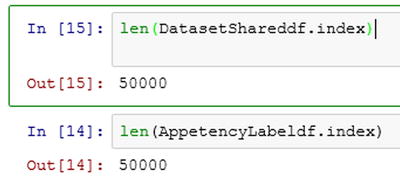
Figure 5-19. Finding the number of rows in each of the dataframes
- You can use the pandas function concat to concatenate the two datasets. To concatenate the two datasets, type the following code into IPython notebook:
import pandas as pd
SharedandAppetencydf = pd.concat(
        [DatasetShareddf,
         AppetencyLabeldf],
         axis=1)
Figure 5-20 shows visually how the two dataframes (DatasetShareddf and AppetencyLabeldf) are concatenated to produce the new dataframe called SharedandAppetencydf.

Figure 5-20. Concatenating dataframes
![]() Note Python provides powerful functions for merging, concatenating, and combining data in the pandas objects (such as DataFrame, Series, and Panel). These functions enable you to perform a join between two datasets (similar to how you perform a join in a relational database), using values from one dataset to patch the values in another dataset.
Note Python provides powerful functions for merging, concatenating, and combining data in the pandas objects (such as DataFrame, Series, and Panel). These functions enable you to perform a join between two datasets (similar to how you perform a join in a relational database), using values from one dataset to patch the values in another dataset.
In this section, you learn how to use Python for concatenating dataframes (for illustration purpose only). You can also use the Add Columns module in ML Studio to concatenate two datasets.
Refer to http://pandas.pydata.org/pandas-docs/stable/merging.html for more examples.
Handling Missing Data Using Python
In this section, you’ll continue using Python for other data wrangling tasks. Specifically, you will use Python to fill in missing values for specific columns, and perform data discretization on the data in some of the columns. You will be using the dataframe that you created in the previous section.
If you have not done that yet, type the following code into IPython notebook. The code uses the azureml module to access the datasets in the ML workspace, and convert them to a dataframe. In Listing 5-1, the workspace_id and authorization_id will be different for your experiments, and you will need to update it with the workspace_id and authorization_id that is provided in the data access code.
Once the SharedandAppetencydf is created, start replacing the missing values. In Python, NaN is the default value used to denote missing data. In this section, you will replace NaN with the value 0. To do this, type the following code in IPython:
df3 = SharedandAppetencydf.fillna(0)
df3[0:5]
You use the fillna() method replace the NaN values with the value 0.
Figure 5-21 shows the first five rows of the datasets after performing fillna(). Notice that NaN has been replaced by 0.

Figure 5-21. Using fillna() on a dataframe
![]() Note For some datasets, exercise caution when replacing a value with 0. This might cause actual rows that contain 0 to become ineffective. Consider adding some constant value (such as 1) to the original dataset before replacing the NaN values.
Note For some datasets, exercise caution when replacing a value with 0. This might cause actual rows that contain 0 to become ineffective. Consider adding some constant value (such as 1) to the original dataset before replacing the NaN values.
Feature Selection Using Python
Feature selection (also known as variable selection) is frequently used by many data scientists to figure out the relevant features that will be useful inputs to an experiment.
By reducing the number of features used, the training time of an experiment can be significantly improved, and it often helps to reduce possibility of overfitting. Most importantly, it enables the model to be simplified, and leads to an easier understanding of the key features that contribute to a prediction.
The Python scikit-learn library provides powerful and comprehensive tools for pre-processing the data and performing model selection, feature selection, dimensionality reduction, and a rich set of machine learning algorithms (including classification, regression, and clustering). The NumPy library empowers Python developers with efficient N-dimensional array capabilities and a rich set of transformation capabilities (Fourier transforms, random number generation, and much more).
In this section, you will learn how to use the dataframes that you defined in the earlier sections of this chapter to determine the most relevant features of the datasets.
Many of the feature selection algorithms require numeric inputs, and it is important to figure out the data types specified in the dataframe. Let’s start by understanding the data types for the data in the dataframe.
- Assuming that you have already defined the dataframe SharedandAppetencydf, type the following code into IPython notebook:
dtypeGroups = df3.columns.to_series().groupby(df3.dtypes).groups
list(dtypeGroups) - After you run the Python code, you will see the list of data types that are used in the dataframe (as shown in Figure 5-22). You can see the different dtypes used, including O (Object), int64, and float64.

Figure 5-22. Data types used in the dataframe
Note pandas supports the use of the following dtypes: float, int, bool, datetime64[ns], timedelta[ns], and object. Each of the numeric dtypes has the item size specified (such as int64, float64). To understand more about pandas dtypes, refer to http://pandas.pydata.org/pandas-docs/stable/basics.html#dtypes. - As a preparation step for feature selection, do the following:
- Select the columns that contain numeric data.
- Specify the labels and features used for feature selection. To do this, copy and paste the following code into the IPython window:
numericdf = df3.select_dtypes(include=['float64'])
labels = df3["target"].values
features = numericdf.values
X, y = features, labels
features.shape
Figure 5-23 shows the output from running the code. The features.shape shows you that there are 50,000 rows and 191 columns that are of type float64. You omit columns of type int64 as features because the only int64 column is the label column.

Figure 5-23. Defining the features and labels used for feature selection
- With the labels and features defined, you are ready to perform feature selection. Various feature selection techniques (such as univariate, L1-based, and tree-based feature selection) are provided in the scikit-learn library. You will use the tree-based feature selection to identify the important features. To do this, type the following code into the IPython notebook:
from sklearn.ensemble import ExtraTreesClassifier

model = ExtraTreesClassifier()
X_new = model.fit(X, y).transform(X)
model
Figure 5-24 shows the model output.

Figure 5-24. Using tree-based feature selection
- Type the following into the IPython notebook to see the number of features selected:
X_new.shapeFigure 5-25 shows that there are 38 columns selected.

Figure 5-25. Number of features selected
- Next, you will use the information on the selected features, and extract the relevant columns from the dataframe df3 (which you defined in an earlier step).
Type the following code into IPython notebook:
import NumPy as np
importances = model.feature_importances_

idx = np.arange(0, X.shape[1])
features_to_keep =
        idx[importances > np.mean(importances)]

df4 = df3.ix[:,features_to_keep]
df5 = pd.concat([df4, AppetencyLabeldf], axis=1)
df5[0:5]
After the code is run, you will see the updated dataframe with 39 columns. The last column is the label column.
Figure 5-26 shows the output from running the Python code.

Figure 5-26. Defining the dataframe, after feature selection
Congratulations! You have successfully performed feature selection on the dataset that you are using in ML studio. IPython notebook provides you with an interactive environment where you can explore data, perform data wrangling, and get the dataset into a shape ready to be used in the subsequent steps in an experiment in ML studio. In the next section, you will learn how to use this in ML Studio.
Running Python Code in an Azure ML Experiment
In the earlier sections, you learned how to access the datasets in your Machine Learning workspace using IPython notebook. The complete code is shown in Listing 5-2.
To use the Python code that you have developed and tested in IPython notebook, use the Execute Python Script module to execute the Python script. During execution, the Execute Python Script module runs on a backend that uses Anaconda 2.1. Because the Python runtime runs in a sandbox, the Python script will not be able to access the network and the local file system on the machine where it is running.
You can either provide the Python script within the module, or you can use a script bundle (similar to how you used a script ZIP bundle when executing an R script). If you have additional Python modules that you plan to use, you should include the additional Python files as part of the ZIP bundle.
When using the Execute Python Script module, the module requires that you specify an entry-point function called azureml_main, and return a single data frame. In order to run the code in Listing 5-3 using the Execute Python Script module, you need to make the following changes:
- You must change the names of the input dataframes. The names of the dataframe for the Execute Python Code module are dataframe1 and dataframe2.
- Depending on the version of Anaconda that you have installed on your local development machine, some functions might not work when running in an Azure ML experiment.
- For example, you can use the select_dtypes function locally, but when used in the Execute Python Script module, an exception is thrown. So change the line
numericdf =
  df3.select_dtypes(include=['float64'])
to
numericdf =
  df3.loc[:, df3.dtypes == np.float64]
Let’s use the modified code given in Listing 5-3 in an Azure ML experiment.
- Using the experiment that you used earlier, drag and drop an Execute Python Script module.
- Connect the CRM Dataset Shared dataset as the first input dataset to the Execute Python Script module.
- Connect the CRM Appetency Labels Shared dataset as the second input dataset to the Execute Python Script module.
- After you have done that, copy and paste the code in Figure 5-27 to the Execute Python Script window. Figure 5-28 shows the completed experiment.

Figure 5-27. Using the Execute Python Script

Figure 5-28. Results dataset after performing feature selection using Python
You are now ready to run the Azure ML experiment, which uses a Python script for feature selection.
- Click Run to start the experiment
- After the experiment has successfully run, you can right-click the Results dataset node to see the features that have been selected. Figure 5-28 shows the four features selected.
- You can also right-click the Python device node to see the output generated when the experiment has completed running the Execute Python Script module. Figure 5-29 shows the output.

Figure 5-29. Python device output
Summary
In this chapter, you learned about the exciting possibilities and scenarios that are enabled by the integration of Python into Azure Machine Learning execute Python scripts from within an ML experiment. Several commonly used Python libraries (pandas, scikit-learn, matplotlib, and NumPy) are available as part of the latest distribution.
You learned how to use these libraries to transform the data from raw data to a finished form. In addition, you learned how to perform data processing, and fill in missing values using IPython notebook. You learned how to integrate Python code that you have developed and tested using IPython notebook, and integrate it as part of an Azure Machine Learning experiment using the Execute Python Script module.