![]()
Building Predictive Maintenance Models
Leading manufacturers are now investing in predictive maintenance, which holds the potential to reduce cost, increase margin and customer satisfaction. Though traditional techniques from statistics and manufacturing have helped, the industry is still plagued by serious quality issues and the high cost of business disruption when components fail. Advances in machine learning offer a unique opportunity to reduce cost and improve customer satisfaction. This chapter will show how to build models for predictive maintenance using Microsoft Azure Machine Learning. Through examples we will demonstrate how you can use Microsoft Azure Machine Learning to build, validate, and deploy a predictive model for predictive maintenance.
Overview
According to Ahmet Duyar, an expert in fault detection and former Visiting Researcher at NASA, a key cause of reduced productivity in the manufacturing industry is low asset effectiveness that results from equipment breakdowns and unnecessary maintenance interventions. In the US alone, the cost of excess maintenance and lost productivity is estimated at $740B, so we clearly need better approaches to maintenance (Duyar, 2011).
Predictive maintenance techniques are designed to predict when maintenance should be performed on a piece of equipment even before it breaks down. By accurately predicting the failure of a component you can reduce unplanned downtime and extend the lifetime of your equipment. Predictive maintenance also offers cost savings since it increases the efficiency of repairs: an engineer can target repair work to the predicted failure and complete the work faster as a result; he/she doesn’t need to spend too much time trying to find the cause of the equipment failure. With predictive maintenance, plant operators can be more proactive and fix issues even before their equipment breaks down.
It is worth clarifying the difference between predictive and preventive maintenance since the two are often confused. Preventive maintenance refers to scheduled maintenance that is typically planned in advance. While useful and in many cases necessary, preventive maintenance can be expensive and ineffective at catching issues that develop in between scheduled appointments. In contrast, predictive maintenance aims to predict failures before they happen.
Let’s use car servicing as an example to illustrate the difference. When you buy a car, the dealer typically recommends regular services based on time or mileage. For instance, some car manufacturers recommend a full service after 6,000 and 10,000 miles. This is a good example of preventive maintenance. As you approach 6,000 miles, your dealer will send a reminder for you to schedule your full service. In contrast, through predictive maintenance, many car manufacturers would prefer to monitor the performance of your car on an ongoing basis through data relayed by sensors from your car to a database system. With this data, they can detect when your transmission or timing belt are beginning to show signs of impending failure and will proactively call you for maintenance, regardless of your car’s mileage.
Predictive maintenance uses non-destructive monitoring during the normal operation of the equipment. Sensors installed on the equipment collect valuable data that can be used to predict and prevent failures.
Current techniques for predictive maintenance include vibration analysis, acoustical analysis, infrared monitoring, oil analysis, and model-based condition modeling. Vibration analysis uses sensors such as accelerometers installed on a motor to determine when it is operating abnormally. According to Ahmet Duyar, vibration analysis is the most widely used approach to condition monitoring, accounting for up 85% of all systems sold. Acoustical analysis uses sonic or ultrasound analysis to detect abnormal friction and stress in rotating machines. While sonic techniques can detect problems in mechanical machines, ultrasound is more flexible and can detect issues in both mechanical and electrical machines. Infrared analysis has the widest range of applications, spanning low- to high-speed equipment as well as mechanical and electrical devices.
Model-based condition monitoring uses mathematical/statistical models to predict failures. First developed by NASA, this technique has a learning phase in which it learns the characteristics of normal operating conditions. Upon completion of the learning phase, the system enters the production phase where it monitors the equipment’s condition. It compares the performance of the equipment to the data collected in the learning phase, and will flag an issue if it detects a statistically significant deviation from the normal operation of the machine. This is a form of anomaly detection where the monitoring system flags an issue when the machine deviates significantly from normal operating conditions.
![]() Note Refer to the following resources for more details on predictive maintenance:
Note Refer to the following resources for more details on predictive maintenance:
http://en.wikipedia.org/wiki/Predictive_maintenance and
Ahmet Duyar, “Simplifying predictive maintenance”, Orbit Vol. 31 No.1, pp. 38-45, 2011.
Predictive Maintenance Scenarios
All predictive maintenance problems are not the same. Hence you need to understand the business problem in order to find the most appropriate technique to use. One size does not fit all! Some of the common scenarios include the following:
- Predicting if a given component will fail or not before it happens. This allows the manufacturer to proactively repair the component before it fails, which in turn reduces unplanned downtime and cost.
- Diagnosing the most likely causes of failure. With this information the manufacturer can be smarter about the repairs. Engineers can fix the problem much faster if they know the most likely causes. And the repair job will be cheaper as a result.
- Predicting when a component will fail. Unlike the first scenario, we need know not just whether a component will fail, but also when the failure is likely to occur. This is important for defining the terms of Service Level Agreements (SLAs) or warranties.
- Predicting the yield failure on a manufacturing plant. This is the subject of this chapter, so let’s explore this more in the next section.
The Business Problem
Imagine that you are a data scientist at a semiconductor manufacturer. Your employer wants you to do the following:
- Build a model that predicts yield failure on their manufacturing process, and
- Through your analysis determine the factors that lead to yield failures in their process.
This is a very important business problem for semiconductor manufacturers since their process can be complex, involving involves several stages from raw sand to the final integrated circuits. Given the complexity, there are several factors that can lead to yield failures downstream in the manufacturing process. Identifying the most important factors helps process engineers improve the yield, and reduce error rates and cost of production, leading to increased productivity.
![]() Note You will need to have an account on Azure Machine Learning. Please refer to Chapter 2 for instructions to set up your new account if you do not have one yet.
Note You will need to have an account on Azure Machine Learning. Please refer to Chapter 2 for instructions to set up your new account if you do not have one yet.
The model we will discuss in this chapter is published as the Predictive Maintenance Model in the Azure Machine Learning Gallery, which you can access at http://gallery.azureml.net/. Feel free to download this experiment to your workspace in Azure Machine Learning.
In Chapter 1, you saw that the data science process typically follows these five steps.
- Define the business problem
- Data acquisition and preparation
- Model development
- Model deployment
- Monitoring model performance
Having defined the business problem, you will explore data acquisition and preparation, model development, evaluation, and deployment in the remainder of this chapter.
Data Acquisition and Preparation
Let’s explore how to load data from source systems and explore the data in Azure Machine Learning.
For this exercise, you will use the SECOM dataset from the University of California at Irvine’s machine learning database. This dataset from the semiconductor manufacturing industry was provided by Michael McCann and Adrian Johnston.
![]() Note The original SECOM dataset is available at the University of California at Irvine’s Machine Learning Repository. This dataset contains 1,567 examples, each with 591 features. Of the 1567 examples, 104 of them represent yield failures.
Note The original SECOM dataset is available at the University of California at Irvine’s Machine Learning Repository. This dataset contains 1,567 examples, each with 591 features. Of the 1567 examples, 104 of them represent yield failures.
The features or columns represent sensor readings from 591 points in the manufacturing process. In addition, it also includes a timestamp and the yield result (a simple pass or fail) for each example. In this donated data, the donors did not provide the actual names of each variable. However, they explain that these variables are collected from sensors or process measurement points in the semiconductor manufacturing plant. These variables include both signal and noise. Your task is to determine which of these factors lead to downstream failures in the process. More details are available at http://archive.ics.uci.edu/ml/machine-learning-databases/secom/secom.names.
For the full dataset also refer to http://archive.ics.uci.edu/ml/machine-learning-databases/secom/.
The data is also available in the Predictive Maintenance Model in the Azure Machine Learning Gallery. If you download this experiment to your workspace, you will also get the dataset automatically, so you can skip the data loading section.
Azure Machine Learning enables you to load data from several sources including your local machine, the Web, SQL Database on Azure, Hive tables, or Azure Blob storage.
For this project, we recommend downloading the Predictive Maintenance Model from the Azure Machine Learning Gallery to your own workspace since it comes with the required dataset. To learn how to load data into Azure Machine Learning, refer to Chapters 2 and 7.
Figure 11-1 shows the first part of the experiment that covers data preparation. The data is loaded and preprocessed for missing values using the Clean Missing Data module. Following this, summary statistics are obtained and the Filter-Based Feature Selection module is used to determine the most important variables for prediction.
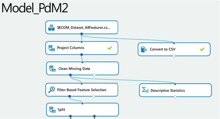
Figure 11-1. Preprocessing the SECOM dataset
Figure 11-2 shows a snapshot of the SECOM data as seen in Azure Machine Learning. As you can see, there are 1,567 rows and 592 columns in the dataset. In addition, Azure Machine Learning also shows the number of unique values per feature and the number of missing values. You can see that many of the sensors have missing values. Further, some of the sensors have a constant reading for all rows. For example, sensor #6 has a reading of 100 for all rows. Such features will have to be eliminated because they add no value to the prediction since there is no variation in their readings.
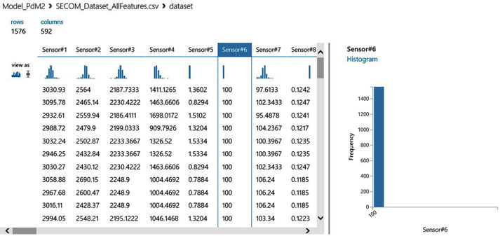
Figure 11-2. Visualizing the SECOM dataset in Azure Machine Learning
Feature Selection
Feature selection is critical in this case since it provides the answer to the second business problem for this project. Indeed, with over 591 features, you must perform feature selection to identify the subset of features that are useful. Through this process you will also eliminate irrelevant and redundant features. With so many features, you run the risk of the curse of dimensionality. If there is a large number of features, the learning problem can be difficult because the many “extra” features can confuse the machine learning algorithm and cause it to have high variance. It’s also important to note that machine learning algorithms are computationally intensive, and reducing the number of features can greatly reduce the time required to train the model, enabling the data scientist to perform experiments in less time. Through careful feature selection, you can find the most influential variables for the prediction. Let’s see how to do feature selection in Azure Machine Learning.
To perform feature selection in Azure Machine Learning, drag the module named Filter-Based Feature Selection from the list of modules in the left pane. You can find this module by either searching for it in the search box or by opening the Feature Selection category. To use this module, you need to connect it to a dataset as the input. Figure 11-3 shows how to use it to perform feature selection on the SECOM dataset. Before running the experiment, use the Launch column selector in the right pane to define the target variable for prediction. In this case, choose the column Yield_Pass_Fail as the target since this is what you wish to predict. When you are done, set the number of desired features to 50. This instructs the feature selector in Azure Machine Learning to find the top 50 variables.
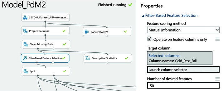
Figure 11-3. Feature selection in Azure Machine Learning
You also need to choose the scoring method that will be used for feature selection. Azure Machine Learning offers the following options for scoring:
- Pearson correlation
- Mutual information
- Kendall correlation
- Spearman correlation
- Chi-Squared
- Fischer score
- Count-based
The correlation methods find the set of variables that are highly correlated with the output, but have low correlation among themselves. The correlation is calculated using Pearson, Kendall, or Spearman correlation coefficients, depending on the option you choose.
The Fisher score uses the Fisher criterion from statistics to rank variables. In contrast, the mutual information option is an information theoretic approach that uses mutual information to rank variables. The mutual information option measures the statistical dependence between the probability density of each variable and that of the outcome variable.
Finally, the Chi-Squared option selects the best features using a test for statistical independence; in other words, it tests whether each variable is independent of the outcome variable. It then ranks the variables using a two-way Chi-Squared test.
![]() Note See http://en.wikipedia.org/wiki/Feature_selection#Correlation_feature_selection or
Note See http://en.wikipedia.org/wiki/Feature_selection#Correlation_feature_selection or
http://jmlr.org/papers/volume3/guyon03a/guyon03a.pdf for more information on feature selection strategies.
When you run the experiment, the Filter-Based Feature Selection module produces two outputs: first, the filtered dataset lists the actual data for the most important variables. Second, the module shows a list of the variables by importance with the scores for each selected variable. Figure 11-4 shows the results of the features. In this case, you set the number of features to 50 and you use mutual information for scoring and ranking the variables. Figure 11-4 shows 51 columns since the results set includes the target variable (Yield_Pass_Fail) plus the top 50 variables including sensor #60, sensor #248, sensor #520, sensor #104, etc. The last row of the results shows the score for each selected variable. Since the variables are ranked, the scores decrease from left to right.
Note that the selected variables will vary based on the scoring method, so it is worth experimenting with different scoring methods before choosing the final set of variables. The Chi-Squared and mutual information scoring methods produce a similar ranking of variables for the SECOM dataset.

Figure 11-4. The results of feature selection for the SECOM dataset showing the top variables
Training the Model
Having completed the data preprocessing, the next step is to train the model to predict the yield. Since the response variable is binary, you can treat this as a binary classification problem. So you can use any of the two-class classification algorithms in Azure Machine Learning such as two-class logistic regression, two-class boosted decision trees, two-class decision forest, two-class neural networks, etc.
![]() Note All predictive maintenance problems are not created equal. Some problems will require different techniques besides classification. For instance, if the goal is to determine when a part will fail, you will need to use survival analysis. Alternatively, if the goal is to predict energy consumption, you may use a forecasting technique or a regression method that predicts continuous outcomes. Hence you need to understand the business problem in order to find the most appropriate technique to use. One size does not fit all!
Note All predictive maintenance problems are not created equal. Some problems will require different techniques besides classification. For instance, if the goal is to determine when a part will fail, you will need to use survival analysis. Alternatively, if the goal is to predict energy consumption, you may use a forecasting technique or a regression method that predicts continuous outcomes. Hence you need to understand the business problem in order to find the most appropriate technique to use. One size does not fit all!
Figure 11-5 shows the full experiment to predict the yield from SECOM data. The top half of the experiment, up to the Split module, implements the data preprocessing phase. The Split module splits the data into two samples, a training sample comprising 70% of the initial dataset, and a test sample with the remaining 30%.
In this experiment, you compare three classification algorithms to find the best prediction of yield. The left branch after the Split module uses the two-class boosted decision tree, the middle branch uses the two-class logistic regression algorithm that is widely used in statistics, and the right branch uses the two-class Bayes Point Machine. Each of these algorithms is trained with the same training sample and tested with the same test sample. You use the module named Train Model to train each algorithm and the Score Model for testing. The module named Evaluate Model is used to evaluate the accuracy of these two classification models.

Figure 11-5. An experiment for predicting the yield from SECOM data
Model Testing and Validation
Once the model is trained, the next step is to test it with a hold-out sample to avoid over-fitting and evaluate model generalization. We have shown how we performed this using a 30% sample for testing the trained model. Another strategy to avoid over-fitting and evaluate model generalization is cross-validation, which was discussed in Chapter 7. By default, Azure Machine Learning uses 10-fold cross-validation. With this approach, you cycle through 10 hold-out samples instead of one for validation. To perform cross-validation for this problem you can simply replace any pair of the Train Model and Score Model modules with the module named Cross Validate Model. Figure 11-6 shows how to perform cross-validation with the Two-Class Logistic Regression portion of this experiment. You will also need to use the whole dataset from the Filter-Based Feature Selection as your input dataset. For cross-validation there is no need to split the data into training and test sets with the Split module since the module named Cross Validate Model will do the required data splits automatically.
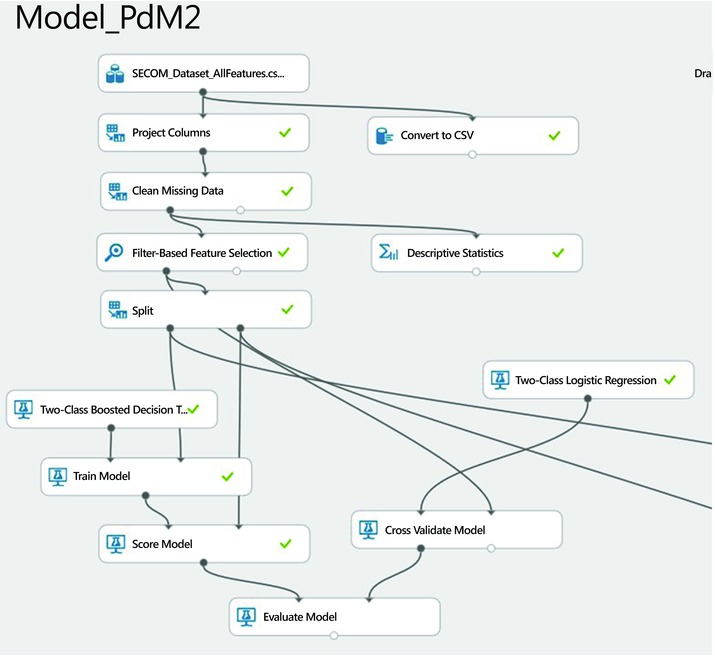
Figure 11-6. A modified experiment with cross-validation
Model Performance
The Evaluate Model module is used to measure the performance of a trained model. This module accepts two datasets as inputs. The first is a scored dataset from a tested model. The second is an optional dataset for comparison. You can use this module to compare the performance of the same model on two different datasets, or to compare the performance of two different models on the same dataset so that you can know which model performs better on the task. After running the experiment, you can check your model’s performance by clicking the small circle at the bottom of the module named Evaluate Model. This module provides the following methods to measure the performance of a classification model such as the propensity model:
- The receiver operating characteristic, or ROC curve, which plots the rate of true positives to false positives
- The lift curve (also known as the gains curve), which plots the number of true positives vs. the positive rate
- The Precision vs. recall chart that shows the model’s precision at different recall rates
- The confusion matrix that shows type I and II errors
Figure 11-7 shows the ROC curve for the model you built earlier. The ROC curve visually shows the performance of a predictive binary classification model. The diagonal line from (0,0) to (1,1) on the chart shows the performance of random guessing, so if you randomly selected the yield, your predictions would be on this diagonal line. A good predictive model should do much better than random guessing. Hence, on the ROC curve, a good model should lie above the diagonal line. The ideal or perfect model that is 100% accurate will have a vertical line from (0,0) to (0,1), followed by a horizontal line from (0,1) to (1,1).
One way to measure the performance from the ROC curve is to measure the area under the curve (AUC). The higher the area under the curve, the better the model’s performance. The ideal model will have an AUC of 1.0, while random guessing will have an AUC of 0.5. The logistic regression model you built has an AUC of 0.758 while the boosted decision tree model has a slightly higher AUC of 0.776! In this experiment, the two-class boosted decision tree had the following parameters:
- Maximum number of leaves per tree = 101 - 900
- Minimum number of samples per leaf = 101 - 900
- Learning rate = 0.1 - 0.9
- Number of trees constructed = 1001 - 9000
- Random number seed = 1

Figure 11-7. Two ROC curves comparing the performance of logistic regression and boosted decision tree models for yield prediction
In addition, Azure Machine Learning also provides the confusion matrix as well as precision and recall rates for both models. By clicking each of the two curves, the tool shows the confusion matrix, precision, and recall rates for the selected model. If you click the bottom curve or the legend named “scored dataset to compare,” the tool shows the performance data for the logistic regression model.
Figure 11-8 shows the confusion matrix for the boosted decision tree model. The confusion matrix has the following four cells:
- True positives: These are cases where yield failed and the model correctly predicts failure.
- True negatives: In the historical dataset, the yield passed, and the model correctly predicts a pass.
- False positives: In this case, the model incorrectly predicts that the yield would fail when in fact it passed. This is commonly referred to as a Type I error. The boosted decision tree model you built had only three false positives.
- False negatives: Here the model incorrectly predicts that the yield would pass when in reality it failed. This is also known as a Type II error. The boosted decision tree model had 30 false negatives.

Figure 11-8. Confusion matrix and more performance metrics
In addition, Figure 11-8 shows the accuracy, precision, and recall of the model. Here are the formulas for these metrics:
Precision is the rate of true positives in the results.

Recall is the percentage of yield failures that the model identifies and is measured as

Finally, the accuracy measures how well the model correctly identifies yield failures and passes, shown as

where tp = true positive, tn = true negative, fp = false positive, and fn = false negative. The F1 score is a weighted average of precision and recall. In this case, it is quite low since the recall is very low.
Techniques for Improving the Model
So given all these metrics, how good is our model? Its accuracy is very high at 93%. Is this good or bad? As you saw in Chapter 7, the accuracy of a model can be misleading especially where there is class imbalance. Please refer to the section entitled “Prioritizing Evaluation Metrics” in Chapter 7 for more details on this.
This specific model is not great. Despite its high accuracy, the model has very low precision, recall, and F1 score. So why is the accuracy is so high? The reason is class imbalance. The SECOM dataset has only 104 cases of yield failure out of 1,567 examples. This is a 6.6% failure rate. With such an imbalanced class even a naïve model can show high accuracy by simply predicting “yield pass” every time. Such a model would have a 93.4% accuracy without correctly identifying a single case of yield failure. With this class imbalance the model learns to predict which cases will pass but fails to learn about yield failures which is the goal of the project.
To address this problem you can use two techniques that will help the classification algorithms to learn the minority class (yield failures): downsampling and upsampling. With downsampling we balance the two classes by reducing the number of cases with yield passes. By reducing the number of passed cases we increase the proportion of yield failures in our sample. This will enable the Machine Learning algorithms to learn to better predict yield failures. With upsampling we use resampling techniques to increase the number of yield failure cases in the data. This also has the effect of increasing the proportion of yield failure cases in our sample, which helps the algorithms to better learn to predict yield failures.
Now let’s explore how you can do upsampling and downsampling in Azure Machine Learning.
![]() Note For more information on upsampling and downsampling refer to the following papers:
Note For more information on upsampling and downsampling refer to the following papers:
Chen, Chao, Liaw, Andy, and Breiman, Leo. “Using Random Forest to learn imbalanced data”. University of California at Berkeley, Department of Statistics. Report Number 666, 2004.
Li, Junyi and Nenkova, A. “Addressing Class Imbalance for Improved Recognition of Implicit Discourse Relations”. Proceedings of the SIGDIAL 2014 Conference, pp. 142–150, Philadelphia, U.S.A., 18–20 June, 2014.
Chawla, N. V., Bowyer, K. W., Hall, L. O., and Kegelmeyer, W. P. (2002). Smote: Synthetic minority over-sampling technique. Journal of Artificial Intelligence Research, 16:321–357.
The SMOTE algorithm in R is in the DMwR package. To use this algorithm you need to install the DMwR package onto your local machine. Detailed instructions for installing any R package into Azure Machine Learning is available on MSDN at http://blogs.msdn.com/b/benjguin/archive/2014/09/24/how-to-upload-an-r-package-to-azure-machine-learning.aspx. We highly recommend this resource if you plan to use the SMOTE implementation from R.
The upsampling technique addresses class imbalance by increasing the number of examples from the minority class. This creates a more balanced dataset with more representation from the minority class. With a more balanced dataset the learning algorithms have a much better chance of learning how to correctly predict the minority class. You can do upsampling easily in Azure Machine Learning using the SMOTE module. This module implements the Synthetic Minority Oversampling TEchnique (SMOTE) developed by Chawla et al. in 2002. This algorithm resolves class imbalance by artificially generating synthetic examples from the minority class using a nearest neighbors approach. The SMOTE algorithm has been implemented in other Machine Learning platforms such as R and WEKA.
In this example, you will use the SMOTE algorithm in R since it does both upsampling and downsampling. You can use this R implementation of the SMOTE algorithm in Azure Machine Learning with the following steps.
First, copy the Predictive Maintenance Model from the Gallery (at http://gallery.azureml.net/) to your workspace.
- The module named Missing Value Scrubber is being deprecated, so replace it with the new module named Clean Missing Data.
- Find the module named Normalize Data and connect its input to the output of the Clean Missing Data module.
- Connect the output of the Normalize Data module to the input of the Filter-Based Feature Selection module
- Drag the new ZIP file containing the DMwR package to the canvas. Also, drag the Execute R Script module to the canvas and insert it after the Split module.
- Connect the DMwR package to the third input of the Execute R Script module. Also, connect the first output of the Split module to the first input of the Execute R Script module.
- Now connect the first output of the Execute R Script module to the second input of the Train Model modules for the Boosted Decision Tree, Logistic Regression, and Bayes Point Machine modules. The result is shown in Figure 11-9.
- Edit the parameters of the Execute R Script module as shown in Figure 11-10. The most critical part is line 24 that calls the SMOTE algorithm with the call
data.set <- SMOTE(Yield_Pass_Fail ~ ., dataset1, k=3, perc.over=300, perc.under=100)
The first parameter is the formula for the prediction problem. In this case the notation Yield_Pass_Fail ~ . denotes that you are trying to predict Yield_Pass_Fail using all input variables.
Dataset1 is the training sample passed to the Execute R Script module.
k=3 instructs SMOTE to use the three nearest neighbors to generate a new synthetic example from the minority class.
perc.over=300 tells SMOTE to create three new failure cases for every example of yield failure in the dataset.
perc.under=100 instructs the SMOTE algorithm to select exactly one case from the majority class for every failure case generated. In this case, it will select three passed examples for every three new failure cases it generates.
- Now run the experiment by clicking the Run button at the bottom of Azure Machine Learning Studio.
- Inspect the results of the experiment as follows.
- Right-click the dot at the bottom of the Evaluate Model module
- Choose Visualize from the menu. The results are shown in Figures 11-11 and 11-12.
Figure 11-11 shows the ROC curve while Figure 11-12 shows the confusion matrix with the accuracy, recall, precision, and F1 score. It is evident that the performance of the Boosted Decision Tree and Logistic Regression models improve after oversampling and undersampling with the SMOTE algorithm. Logistic Regression performs better than Boosted Decision Tree after oversampling and undersampling. Although accuracy and precision decrease, recall rate increases from a mere 3.2% to 78.9% while the F1 score also increases from 5.7% to 23.4. Area Under the Curve (AUC) decreases slightly from 77.6% to 75.1%.

Figure 11-9. The modified Predictive Maintenance Model with the added Execute R Script module and the DMwR package
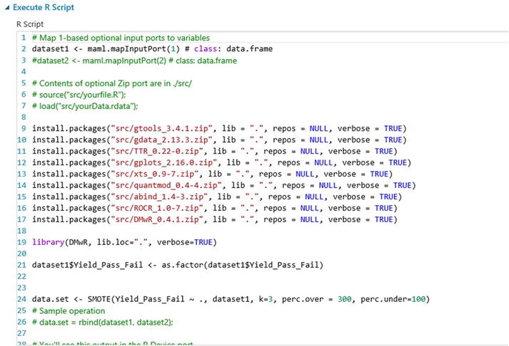
Figure 11-10. Invoking the SMOTE algorithm in the DMwR package from the Execute R Script module in Azure Machine Learning
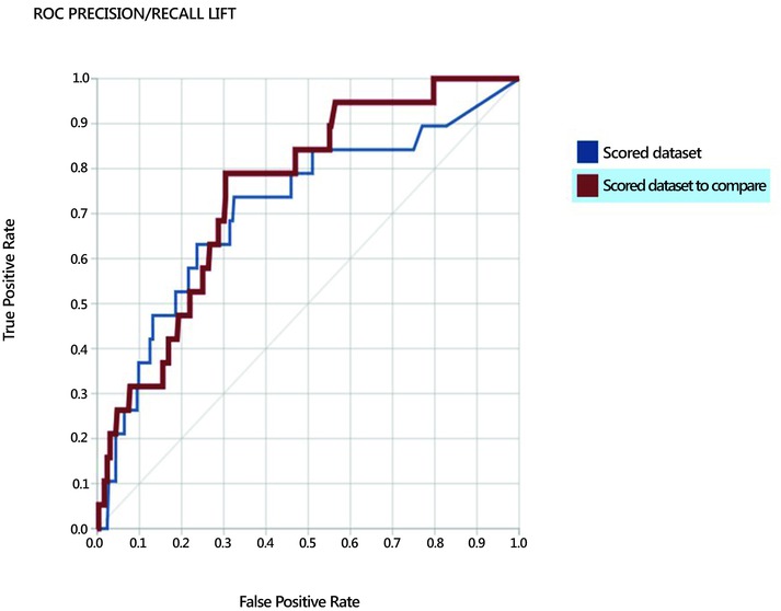
Figure 11-11. The ROC curves of the Boosted Decision Tree and Logistic Regression models after upsampling and downsampling with the SMOTE algorithm in R

Figure 11-12. The confusion matrix, precision, recall, and F1 score of the Boosted Decision Tree model after upsampling and downsampling with the SMOTE algorithm in R
Model Deployment
When you build and test a predictive model that meets your needs, you can use Azure Machine Learning to deploy it into production for business use. A key differentiator of Azure Machine Learning is the ease of deployment in production. Once a model is complete, it can be deployed very easily into production as a web service. Once deployed, the model can be invoked as a web service from multiple devices including servers, laptops, tablets, or even smartphones.
The following two steps are required to deploy a model into production.
- Create a predictive experiment, and
- Publish your experiment as a web service.
Let’s review these steps in detail and see how they apply to your finished model built in the previous sections.
Creating a Predictive Experiment
To create a predictive experiment, follow these steps in Azure Machine Learning Studio.
- Run your experiment with the Run button at the bottom of Azure Machine Learning Studio.
- Select the Train Model module in the left branch containing the Boosted Decision Tree. This tells the tools that you plan to deploy the Boosted Decision Tree model in production. This step is only necessary if you have several training modules in your experiment.
- Next, click Set Up Web Service | Predictive Web Service (Recommended) at the bottom of Azure Machine Learning Studio. Azure Machine Learning will automatically create a predictive experiment. In the process, it deletes all the modules that are not needed. For example, all the other Train Model modules, the Split, Project, and other modules are removed. The tool replaces the Two-Class Boosted Decision Tree module and its Train Model module with the newly trained model. It also adds a new web input and output for your experiment.
Your predictive experiment should appear as shown Figure 11-13. You are now ready to deploy your new predictive experiment in production. To do this, let’s move to the next step.

Figure 11-13. The scoring experiment ready for deployment as a web service
Publishing Your Experiment as a Web Service
At this point your model is now ready to be deployed as a web service. To do this, follow these steps.
- Run your experiment with the Run button at the bottom of Azure Machine Learning Studio.
- Click the Deploy Web Service button at the bottom of Azure Machine Learning Studio. The tool will deploy your scored model as a web service. The result should appear as shown in Figure 11-14.
Congratulations, you have just published your machine learning model into production. Figure 11-14 shows the API key for your model as well as the URLs you will use to call your model either interactively in request/response mode, or in batch mode. It also shows a link to a new Excel workbook you can download to your local file system. With this spreadsheet you can call your model to score data in Excel. See Chapter 8 for details on how to visualize your results with this Excel workbook. In addition, you also get sample code you can use to invoke your new web service in C#, Python, or R.

Figure 11-14. The results of the deployed model showing the API key, URLs for the service, and a link to a new Excel workbook you can download
Summary
You began this chapter by exploring predictive maintenance, which shows the business opportunity and the promise of machine learning. Using the SECOM semiconductor manufacturing data from the University of California at Irvine’s Machine Learning Data Repository, you learned how to build and deploy a predictive maintenance solution in Azure Machine Learning. In this step-by-step guide, we explained how to perform data preprocessing and analysis, which are critical for understanding the data. With that understanding of the data, we used a two-class logistic regression and a two-class boosted decision tree algorithm to perform classification. You also saw how to evaluate the performance of your models and avoid over-fitting. We explored how to use upsampling and downsampling to significantly improve the performance of your predictive model. Finally, you saw how to deploy the finished model in production as a machine learning web service on Microsoft Azure.