1

Three Ways to Determine the Discount Rate

In this chapter, we present the simple two-period model that is used in classical economics textbooks to examine the problem of consumption, saving, and investment in a competitive economy. This model reminds us of the key role of the interest rate for the determination of economic growth. Its equilibrium level balances the demand and the supply of liquidity, which are themselves characterized by time preferences and investment opportunities. From a simple arbitrage argument, any new investment opportunity in the economy should be evaluated by using the interest rate as the rate at which the future benefits of the project should be discounted.

DESCRIPTION OF THE ECONOMY

Let us consider a simple economy composed of several identical individuals who live for two periods, “today” and “the future.” These periods are indexed respectively by 0 and t. At the beginning of the first period, each agent is endowed with a quantity w of the single consumption good. Let us call this good “rice.” Rice can be consumed immediately, or it can be planted to produce a crop in the future. This means that rice is also an asset, a form of capital yielding a benefit for the future. Let us assume that planting k units of rice today yields f(k) units of grain in the future. We assume that function f is increasing and concave, and that f(0) = 0. The derivative of f is the marginal productivity of capital, which is thus assumed to be positive and decreasing.

How should these individuals allocate their initial endowment of rice between immediate consumption and saving/investment for the future? In order to answer this question, it is necessary to first determine the consumers’ lifetime objective. At this stage, the general view is taken that they evaluate their lifetime utility as U(c₀, c_t), where c₀ and c_t are the level of consumption of rice today and in the future respectively. The bivariate utility function U is assumed to be increasing in its two arguments. Increasing consumption increases welfare. It is also assumed to be concave. This implies in particular that the marginal utility of rice in periods 0 or t is decreasing. The effect on welfare of one more grain of rice is larger when the consumption level is low than when it is high. The concavity of U also implies that there is a preference for consumption smoothing over time. If the two consumption plans (c₀, c_t) = (1,3) and (3,1) are equaly preferred, then the consumption plan (2,2) is certainly preferred to either of them.

OPTIMAL CONSUMPTION PLAN

It is possible to use the standard graphical representation of this problem. In figure 1.1, the set of feasible consumption plans has been drawn in a Fisher diagram. It is represented by the grey area whose upper frontier is represented as the locus of consumption plans (w – k, f (k)): When k is saved from the initial endowment w of rice, one can consume c₀ = w – k in the first period, and c_t = f(k) in the second period. Because of decreasing marginal productivity of capital, this feasibility frontier is concave. Also represented is the indifference curve defined by equation U(c₀, c_t) = U_A that is tangent to this feasibility frontier. Because U is concave, indifference curves are convex. All plans represented by points above this curve yield an intertemporal welfare that is larger than U_A. It clearly appears that the preferred consumption plan in the feasible set is consumption plan A, which yields an intertemporal welfare U_A. There is no feasible consumption plan that generates a level of intertemporal welfare larger than that.

The optimal consumption plan A is characterized by the tangency of the feasibility frontier and the indifference curve. Technically, it is written as

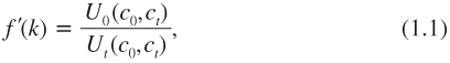
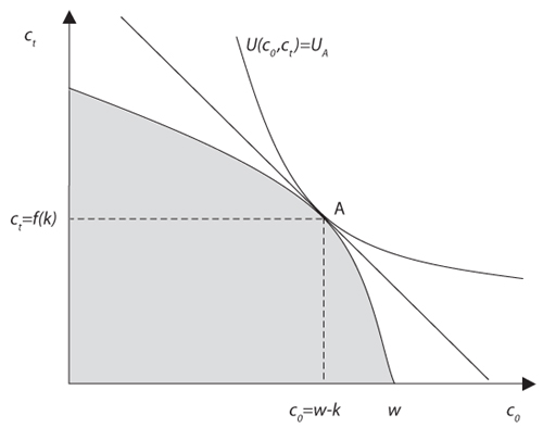
Figure 1.1. The optimal consumption plan in a Fisher diagram

where U_i is the partial derivative of U with respect to c_i. Condition (1.1) is the first order condition of the problem of maximizing U(w – k, f (k)) with respect to k. The left-hand side of equation (1.1) is the marginal productivity of capital or the increase in future consumption when one more unit of rice is invested today in the productive capital of the economy. It measures the (absolute value of the) slope of the feasibility frontier, evaluated at A. The right-hand side of this equality is the marginal rate of substitution between current and future consumption, or the welfare-preserving return on saving. This intertemporal marginal rate of substitution tells us by how much future consumption must be increased to compensate for the sacrifice of one unit of current consumption. It measures the (absolute value of the) slope of the indifference curve at A.

Condition (1.1) has a simple economic intuition. It states that at the optimum, one additional grain of rice planted today yields an increase f′(k) in the future consumption of rice which is just sufficient to compensate for the marginal sacrifice of this grain of rice not consumed today. If another plan on the feasibility frontier to the southeast of A were selected, where k is smaller, the same sacrifice today yields a future benefit that more than compensates for the initial sacrifice. This is because the smaller k implies at the same time a larger marginal productivity of capital and a smaller marginal rate of substitution. The latter arises from the fact that to the southeast of A, consumption is very unequal over time, which implies that one is ready to sacrifice more for the future. Symmetrically, in the northwest section of the feasibility frontier where k is larger than at A, the marginal productivity is small, and the marginal rate of substitution is large. It implies that a reduction of k yields an increase in intertemporal welfare.

THE INTEREST RATE

Because all individuals are assumed to have the same initial endowment and the same intertemporal preferences, they will all select consumption plan A in autarky. Suppose that a frictionless credit market opens, in which agents can exchange one unit of rice today against the commitment to deliver R units of rice in the future, where t is the number of years between the present and the future. In the absence of any solvency problem,¹ one can interpret R as the gross interest rate in the economy. Because agents have the possibility to transfer wealth by investing in their own rice technology, a simple arbitrage argument leads to the conclusion that

To show this, suppose that this equality did not hold and that R was larger than the marginal productivity of capital. This would imply that all agents would be willing to reduce their investment in their own rice technology to invest in the credit market that yields a larger return. This would induce an excess supply of credit on financial markets. This cannot be an equilibrium. The interest rate would go down. Symmetrically, if R was smaller than the marginal productivity of capital, all agents would like to get a loan to invest in rice production. This cannot be an equilibrium either. Thus, condition (1.2) characterizes the unique equilibrium on credit market. We conclude that the competitive equilibrium on financial markets is such that the interest rate equals the rate of return of productive capital in the economy.

The existence of a credit market transforms the individual feasibility condition represented by the grey area in figure 1.1 by a budget constraint corresponding to the straight line in the same figure. Its slope equals –R. By construction, this transformation of the constraint faced by each consumer in the economy does not change their optimal consumption plan.

THE DISCOUNT RATE

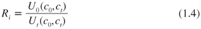
Let us now consider the crucial question this book addresses. Suppose that an entrepreneur, the government, or a consumer is contemplating a new collective investment project. This project has an initial cost ε unit of rice per capita, and it will yield a sure benefit εR_i unit of rice per capita in the future. Variable R_i can be recognized as the internal gross rate of return of the project. In our framework, in which the single consumption good is rice, this investment project could be using a fraction of the initial endowment in rice to manipulate some of the rice’s genes, yielding an improved rice production technology. However, this section can be applied more generally to investment projects in a more complex economy. How should projects such as new transportation infrastructure, investments in education, or fighting climate change be valued?

What is the minimum rate of return of the project under scrutiny that would make it desirable from the collective point of view? The answer to this question is usually referred to as the efficient discount rate. Is it necessary to know how the initial cost of an investment will be financed to characterize it? Does it matter whether the initial cost of the project will be financed by a corresponding reduction in the level of current consumption or by a corresponding reduction in everyone’s investment in their own rice production technology?

Suppose first that the initial cost is financed by a reduction in the level of initial consumption. How does this collective investment modify the people’s intertemporal welfare? Because we assume that ε is small, one can use standard differential calculus to obtain

To get the minimum rate of return that makes the project socially desirable, one should equalize ΔU to zero. This implies that the socially efficient discount rate R_i is such that

This means that the efficient discount rate is equal to the welfare-preserving return on saving.

Suppose alternatively that the collective investment project is financed by a corresponding reduction in the productive capital in the economy. Trivially, the project is socially desirable only if its internal rate of return is larger than the marginal return of productive capital in the economy. This seemingly innocuous observation is important and is deep-rooted in the brain of most economists: evaluations must also be made by comparisons, and one should take into account the opportunity cost of funds. This means that the discount rate must equal the rate of return of capital: R_i=f′(k). This condition guarantees that the marginal investment project is socially at least as good as investing in the productive capital in the economy. Requiring that the Net Present Value (NPV) of a project is positive is equivalent to checking that this project does better for the future than all other unfunded projects available in the economy.

Because consumption plans are optimized, we know that f′(k)=U₀/U_t. When calculating the socially efficient discount rate, it is in fact irrelevant whether the initial cost is financed by a reduction in consumption or in other productive investments. To sum up, it has been shown that

Notice that we could have gone straight to the point that the efficient discount rate must be equal to the interest rate by observing that any agent can finance the initial cost ε by borrowing it today on the credit market. This will yield a reimbursement at date t equaling εR, where R is the interest rate. Obviously, the project is efficient if its benefit at date t net of this reimbursement—which is referred to as the Net Future Value (NFV)—is non-negative. The critical internal rate of return is thus defined as yielding a zero NFV:

This rule is better known as the NPV rule by dividing the above equality by R:

which holds if and only if R_i = R. This is a very natural approach for any specific economic agent. When assessing a project, she does not need to know whether the investment will crowd out other investments, or whether it will reduce aggregate consumption in the economy.

CONTINUOUSLY COMPOUNDED RATES

In this chapter, as in most of this book, we consider discrete-time models. However, we will hereafter use continuously compounded interest rates and rates of return. For example, consider as previously stated a credit contract in which the borrower must repay R units of rice in t years per unit of rice borrowed today. At which rate ρ does the debt grow over time from 1 to R between dates 0 and t? If one wants this rate to be constant, it must be defined by exp(ρt) = R, or

Notice that ρ is the continuously compounded interest rate, whereas R is the gross interest rate between 0 and t. In the same fashion, we can define respectively the (continuously compounded) rate of return of capital at the margin and the welfare-preserving rate of return of saving as follows:

Parameter ρ_u characterizes the minimum rate of return on an investment of duration t to at least maintain intertemporal welfare. In this chapter, we have shown that the discount rate must be equal to ρ = ρ_k = ρ_u.

AN INTERGENERATIONAL PERSPECTIVE

Earlier in this chapter, we implicitly considered private investment projects without externalities. Consider alternatively collective projects that have impacts over several generations of consumers. In this context, we can identify c₀ as the consumption level of the current generation, and c_t as the one of the future generation living in period t. When generations’ lifetimes do not overlap, credit markets will not be operational. There is just no way for future generations to compensate current ones for the sacrifices that the later could be requested to make. Some forms of exchange can be organized on credit markets among different generations that overlap with each other, but it is intuitive that the equilibrium observed in this economy will not be efficient. Overlapping Generations (OLG) models were first examined by Allais (1947), Samuelson (1958), and Diamond (1965). The existence of OLG implies that consumption plans are not socially efficient, and that the interest rate observed on financial markets should not be used as a driver to evaluate public policies impacting several generations.

When different generations bear the costs and the benefits of the investment under scrutiny, the utility function U considered in the chapter should be reinterpreted as the social welfare function. This tranforms our descriptive approach into a prescriptive one. In this framework, U characterizes the collective preferences toward the allocation of consumption across generations. It should be used to evaluate collective investment projects. Consumption plan A in figure 1.1 represents the socially efficient solution, but is generally not a competitive equilibrium.

SUMMARY

This chapter has shown that the socially efficient discount rate can be estimated in three different ways:

1.  The discount rate is the interest rate observed on financial markets. This interest rate reveals important information about society’s willingness to transfer wealth to the future.

2.  The discount rate is the rate of return on marginal productive capital in the economy. Indeed, one should invest in a new project only if its rate of return is larger than alternative opportunities to invest in productive capital.

3.  The discount rate is the welfare-preserving rate of return on savings. Investment reduces current consumption and therefore has a negative impact on welfare. However, the investment will increase consumption and therefore has a positive impact on intertemporal welfare. One should invest in a new project only if the reduction in welfare due to the immediate sacrifice is more than compensated for by the increase in welfare due to the future benefit.

It has also been shown that these three definitions of the discount rate are fully compatible with each other when consumption plans are optimized and credit markets are frictionless.

REFERENCES

Allais, M. (1947), Economie et intérêt, Imprimerie Nationale et Librairie des Publications Officielles, Paris.

Diamond, P. (1965), National debt in a neoclassical growth model, American Economic Review, 55, 1126–1150.

Samuelson, P. A. (1958), An exact consumption-loan model of interest with or without the social contrivance of money, Journal of Political Economy 66(6), 467–482.

¹ The existence of a really risk-free asset in the economy may be questioned. Most sovereign debts contain a default risk. Moreover, their returns are rarely indexed on inflation, so that an inflation risk should be included in the picture. See chapter 7.