6

Parametric Uncertainty and Fat Tails

This book started the analysis of discount rates by considering a sure rate of growth of consumption. The analysis was extended by recognizing that economic growth is uncertain. In the previous chapter, it was noted that the parameters governing this uncertainty may be unstable. In this chapter, we go one step further by recognizing that the probability distribution for economic growth is itself subject to some parametric uncertainty.

Estimation of the parameters governing a stochastic process, such as the mean or the volatility, can be performed using a data set of past realizations of this process. However, this sample may not contain all possible scenarios that could occur in the future. For example, until the early 1970s, the Mexican currency was pegged to the dollar, so that the estimation of trend and volatility of the exchange rate of the peso were close to zero. Thus, the econometric analysis suggested a very small exchange risk. Based on this data it was therefore quite hard to explain the large premium which was observed between Mexican and U.S. interest rates. This was called the “peso problem.” The sharp devaluation of the peso in 1976 provided the solution to the puzzle: the data did not contain this small probability event, although most investors had it in mind.

In a similar way to the peso problem, there is a limited data set for the dynamics of economic growth. The absence of a sufficiently large data set to estimate the long-term growth process of the economy implies that its parameters are uncertain and subject to learning in the future. This problem is particularly crucial when its parameters are unstable, or when the dynamic process entails low-probability extreme events. The rarer the event, the less precise is our estimate of its likelihood. This builds a bridge between the problem of parametric uncertainty, and the one of extreme events.

UNCERTAIN GROWTH

Suppose that the dynamic process c₀, c₁, c₂, … is a function of a parameter θ. The true value of θ is unknown. For the sake of simplicity, suppose that θ can take n possible values θ = 1, …, n. Our prior beliefs about θ at date 0 are characterized by a probability distribution (q₁, …, q_n), q_θ > 0, Σq_θ = 1, where q_θ is the probability that the true value of the parameter be θ. By the law of iterated expectations, we have that

It implies that the pricing formula (4.1) can be rewritten as

Let r_tθ denote the discount rate that would be efficient for horizon t if we knew for sure that the true value of the parameter was θ. This means that r_tθ is defined as

Combining equations (6.2) and (6.3) yields that

In other words, the socially efficient discount factor under parametric uncertainty equals the expectation of the conditionally efficient discount factors (the discount factors that would be efficient for each value of the parameter if it was known with certainty).

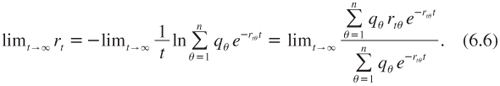
Notice that the expectation concerns the discount factors, not the discount rates. In fact, the socially efficient discount rate defined by (6.4) can be interpreted as the certainty equivalent rate of the uncertain rates r_tθ, θ = 1, …, n, under the implicit utility function h(r) = –exp(–rt). This function is increasing and concave, with an index of concavity measured by t. It implies that the certainty equivalent r_t is smaller than the mean of the uncertain r_tθ. However, at the limit, we obtain

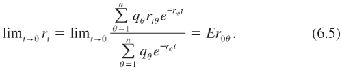
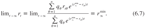
Moreover, as long as the support of r_tθ remains bounded, r_t tends to the lower bound of this support when t tends to infinity. Indeed, using L’Hopital’s rule, we have that

Let denote the smallest possible discount rate when t tends to infinity: = lim_t→∞ min_θr_tθ. Then, the previous equation implies that

The rate at which cash flows occurring in the short term should be discounted is equal to the expectation of the conditionally efficient discount rate. Moreover, as long as the support of r_tθ remains bounded, r_t tends to the lower bound of this support when t tends to infinity. In order to get an intuition for these results, let us examine the simplest case when the stochastic process governing ln c_t is a random walk conditional on θ.

CONDITIONAL ON θ, THE GROWTH PROCESS IS A RANDOM WALK

A special case of the model we mentioned is as follows:

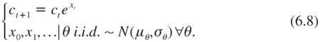
This is a discrete version of an arithmetic Brownian motion with an unknown trend and/or volatility. Although this process is a random walk conditional on θ, x_t exhibits some serial correlation. Suppose for example that only the trend μ_θ is subject to parametric uncertainty. Then, using Bayes’ rule, the observation of a large x₀ yields an upward revision to beliefs about the trend of economic growth.

Conditional on θ, the dynamic process of x_t is a normal random walk. As seen before, equation (6.3) has an analytical solution in that case:

In particular, r_tθ is independent of t. Under the hidden structure characterized by (μ_θ, σ_θ), θ = 1, …, n, the term structure of the socially efficient discount rate is obtained by rewriting equation (6.4) as follows:

The socially efficient discount rate under this parametric uncertainty is equal to the expected value of r_θ = δ+γμ_θ-0.5γ² for short maturities, is decreasing with t, and tends to the smallest possible value of r_θ when t tends to infinity.

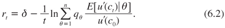
Following Gollier (2008), the intuition for these results is based on the observation that the parametric uncertainty plays a crucial role in shaping the uncertainty surrounding consumption in the distant future. To illustrate this, let us assume that the volatility of the growth of log consumption is known and equal to σ = 3.6%, but the trend μ is unknown. It can be either 1% or 3% with equal probability. In figure 6.1, we draw the distribution of lnc_t/c₀ for t = 1, 10, and 100. Ex ante, the distribution of lnc₁/c₀ is a mixture of two normal densities. However, the uncertainty affecting the trend is a second-order source of uncertainty compared to the volatility of the growth rate. So, in the short run, assuming a trend of (1% + 3%)/2 to determine the efficient discount rate is a good approximation. In contrast, the uncertainty affecting consumption in one century’s time is mostly a result of the uncertainty over the growth trend. Conditional on the growth trend, μ = 1% or μ = 3%, the expectation of c₁₀₀/c₀ is exp(100(μ + 0.5 × 0.036²)), which equals 3.5 or 26. The magnitude of the uncertainty from this source can be compared to that from the intrinsic volatility of growth. Assuming μ = 2% and σ = 3.6%, the 95% confidence interval for lnc₁₀₀/c₀ is [1.29, 2.71].

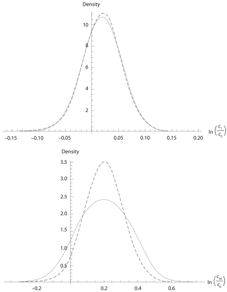
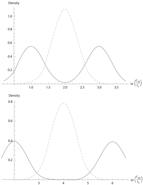
Figure 6.1. Density function of lnc_t/c₀ for t = 1, 10, 100, and 200, under the assumption that μ ~ (1%, 1/2; 3%, 1/2) and σ = 3.6%. The dashed curve is the density function without parametric uncertainty and μ = 2%.

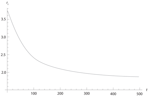
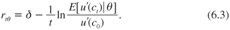
Figure 6.2. Efficient term structure with μ ~ (1%, 1/2; 3%, 1/2), σ = 3.6%, δ = 0%, and γ = 2.

The bottom line is that parametric uncertainty entails fatter tails for the distribution of future consumption. The thickness of the tails increases with the time horizon. Integrating out parameter uncertainty by Bayes’ rule spreads apart probabilities and thickens the tails of the posterior distribution for predicting the future growth rate of consumption. This explains why the term structure of discount rates is decreasing. Indeed, the growing gap of uncertainty, compared to the random walk hypothesis with the mean trend, magnifies the precautionary effect in the distant future. We get a decreasing term structure because the precautionary effect tends to reduce the discount rate. In the long run, the fear of a low economic growth rate of 1% dominates all other considerations about how to value the future. Under the assumption that δ = 0% and γ = 2, the discount rate converges to r_∞ = 2 × 1% –0.5 × 2² × 0.036² = 1.7%, as shown in figure 6.2.

THE CASE OF AN UNKNOWN TREND OF ECONOMIC GROWTH

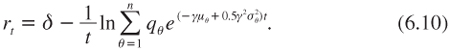
When the growth of log consumption conditional on θ is normally distributed, the term structure of efficient discount rates is characterized by equation (6.10), which is rewritten as follows:

Hereafter θ is allowed to have a continuous distribution. In this section, it is supposed that the volatility of the growth rate of consumption is known, so that σ_θ = σ for all θ. However, more sophisticated prior distributions for µ_θ are considered than the two-state case from the previous section. Suppose that µ_θ is normally distributed with mean µ₀ and variance can be interpreted as a measure of the degree of uncertainty about the true growth of log consumption. Observe from (6.11) that once again this is a situation requiring the expectation of the exponential of a normally distributed random variable to be computed. Using lemma 1, it is obtained that:

This expression can alternatively be derived from the well-known property that if the conditional distribution ln c_t/c₀ given (µ, σ) is normal with mean µt and variance σ²t, and if µt is itself normally distributed with mean µ₀t and variance then the unconditional distribution of ln c_t/c₀ is also normal with mean µ₀t and variance Define as the expected growth rate of consumption in the time interval [0, t ]. This allows equation (6.12) to be rewritten as

The term structure of efficient discount rates (6.13) is linearly decreasing in maturity, t. It tends to min r_θ = –∞ when t tends to infinity. The support of r_θ is unbounded below because the expected growth of log consumption is normally distributed. The possibility that the true growth trend for the economy is a large negative number is central to the valuation of distant cash flows. Although the probability of such an event may be very small, the scenario of a vanishing GDP per capita is greatly feared by the representative agent. When combined with the property that lim_c→0u′(c) is infinite for power utility functions, it implies that there is a very high social value for transfers of wealth to distant dates where there is the possibility of close to zero per capita consumption.

One can question the normality of the prior beliefs on the trend of log consumption, or more generally the nature and origin of these prior beliefs. It is possible to approach these questions by using Bayesian inference. Suppose that our current beliefs about the future growth of the economy combines primitive beliefs about it—which may be uninformative—and the observation of a sample of T past realizations of growth of log consumption (x_–T, …, x_–1). Suppose that the primitive beliefs take the form of three assumptions. First, changes in log consumption are independent and normally distributed. Second, the variance of the change in log consumption is a known constant σ². Third, the mean µ of the change in log consumption is normally distributed with mean µ^* and variance σ^*2. The observation of the recent changes (x_–T, …, x_–1) affects these beliefs. Using Bayes’ rule, it follows that

It is well-known that this process of revising beliefs yields a posterior distribution for the change in ln c which is normally distributed with mean:

where m = T^–1–Tx_τ is the sample mean for changes in ln c. See for example Leamer (1978, theorem 2.3). The new expected growth, µ₀, is a weighted average of the prior expectation and of the sample mean. A large sample mean pushes beliefs upward. The sensitiveness of posterior beliefs is an increasing function of the relative precision (σ²/T)^–1 of the sample information relative to the precision (σ^–2* of prior beliefs. The posterior variance of μ is equal to

The posterior (µ₀, σ₀) can then be considered as the updated mean and standard deviation for the change in log consumption. It can be plugged into equation (6.12) to determine the socially efficient discount rates. A special case arises when the prior beliefs are uninformative. This can be approximated by assuming that σ^* is very large. Equations (6.15) and (6.16) then become

In this case, the beliefs at date 0 are entirely determined by the observation of economic growth. They are normal, with mean and variance given by (6.17). This is the standard way of justifying a normal distribution for the prior beliefs. Notice that this yields a linearly decreasing term structure.

THE CASE OF AN UNKNOWN VOLATILITY OF ECONOMIC GROWTH

In a sequence of two recent papers, Weitzman (2007, 2009) considers an alternative model in which the unknown parameter for the distribution of ln c_t+1/c_t is its volatility rather than its mean. Suppose that µ_θ = µ for all θ. The plausible distribution for the volatility must of course have its support in ₊, which excludes the normal distribution. As has already been observed, it is often more convenient to work with the precision, p_θ = , rather than the variance. When the precision is unknown, it is standard in the literature to assume that it has a gamma distribution: p_θ ~ Γ(a,b). The gamma distribution has two parameters, a shape parameter a > 0, and a scale parameter b > 0. Its density function is

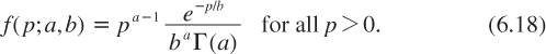
The gamma function extends the factorial one to non-integer numbers, with Γ(a) = (a–1)! when a is a natural integer.

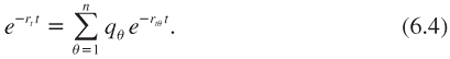
The mean and variance of p_θ are respectively equal to ab and ab². Remember that the observed volatility of yearly changes in log consumption is around 3.6%, which gives a precision of approximately (0.036)^–2 ≈ 800. In figure 6.3, four different gamma densities are drawn, all with the same mean ab = 800.

The remaining challenge is to determine the shape of the term structure of discount rates under this specification. It is characterized by equation (6.11) which is rewritten as follows:

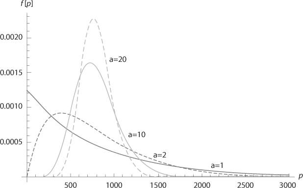
Figure 6.3. Gamma densities for different parameters (a, b) with the same Ep = ab = 800.

The integral in this equation is unbounded. It is the moment-generating function evaluated at 0.5γ²t for the random variable 1/p, which has an inverted-gamma distribution. The precautionary effect is infinite, independent of the degree of parametric uncertainty!

An alternative way to view this problem is achieved by characterizing the unconditional distribution of x_t. Conditional on σ_θ, it is normal. Combining a normal distribution of mean m with a gamma distribution Γ(a, b) for its uncertain precision yields an unconditional distribution that is a Student’s t- distribution. This distribution has v = 2a degrees of freedom, with mean μ and variance 1/(a – 1)b:

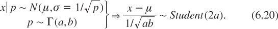
The Student’s t-distribution has fatter tails than the corresponding normal distribution with the same mean and variance. In figure 6.4, we draw different unconditional distributions for the annual change in log consumption by using the same parameters of the gamma distribution as in the previous figure: (a,b) = (1,800), (2,400), (10,80), and (20,40). We assume that x has a mean of µ = 2%, so that (x–0.02)√800 is a Student’s t-distribution with 2a degrees of freedom. When a tends to infinity, the Student’s t-distribution tends to normal. However, a finite parameter a has the effect of thickening the tails of the distribution compared to the normal one. Just as for other sources of parametric uncertainty, the parametric uncertainty about the volatility of the growth process makes the distribution of the growth rate riskier.

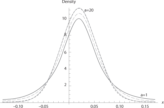
Figure 6.4. Density functions for the change in log consumption. We assume that (x – 0.02)√800 is a Student’s t-distribution with 2a degrees of freedom, a = 1, 2, 10 and 20. The dashed curve is the density of N(0.02, 1/√800).

The differences between the normal distribution and the Student’s t-distribution may look quite marginal in figure 6.4. However, the tails of the distributions are significantly different. There is relatively much more probability mass in the Student’s t-distribution than in the normal one. Let us define function g(t;v) as the ratio of probabilities that x_S(v) and x_N are smaller than t, where x_S(v) and x_N are respectively the Student’s t-distribution with v degrees of freedom, and the standardized normal distribution:

TABLE 6.1.
Ratio g(t;v) of probabilities in the left tail

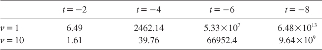
Table 6.1 shows how big g can be in the left tail.

What is special with this specific parametric uncertainty is that the tails of the unconditional distribution of x are particularly thick. They are so thick that the precautionary effect becomes infinite. This can be checked in the following way. We have that

Where M_x(k) = Ee^xk is the moment-generating function of random variable x. For x ~ N(µ,θ), we know that M_x(k) = exp(µk+0.5σ²k²). However, the Student’s t-distribution has an unbounded moment-generating function. Therefore, r₁ = –∞

It can be argued that this result is driven by the fact that “too much” parametric uncertainty is contained in the gamma distribution for the precision p. This point again raises the question of the status of our beliefs about the distribution of the uncertain parameter. Suppose that the only source of information is the observation of the past volatility of economic growth. Suppose that the true distribution of x_t is normal. Using Bayes’ rule, it can be proved that updating the normal-gamma prior beliefs using the observation of (x_–T, …, x_–1) yields a normal-gamma posterior belief (see Leamer 1978, theorem 2.4). In particular, if µ is known and if the prior on σ is uninformative, the posterior distribution of p = 1/σ² must be a gamma distribution. Thus, the use of an inverse-gamma distribution for the precision is a natural way to model the uncertainty affecting the variance of a Brownian process.

The unboundedness of the efficient discount rate in this case is a consequence of the Inada property u′(0) = +∞ of the utility function, and from the standard marginalist approach to economic valuation. The representative agent places enormous value on any investment that yields a sure consumption, ε > 0, in the future. Once these investments are implemented, the probability that future consumption will fall below ε > 0 will be zero, and the discount rate will be bounded.

SUMMARY OF MAIN RESULTS

1.  A simple way to generate a decreasing structure of discount rates is to recognize that some parameters of the consumption growth process are uncertain. Parametric uncertainty about the trend is of limited importance in the short run, but in the long run is of huge significance. In particular, it tends to magnify the long term risk (fatter tails) and the associated precautionary effect for long horizons.

2.  For each time horizon, the efficient discount factor is the expected value of the efficient discount factors conditional to each plausible value of the parameters. As a consequence, for distant futures, the efficient unconditional discount rate tends to the smallest plausible conditional discount rate.

3.  Suppose that consumption follows a geometric Brownian motion with an uncertain trend. If this trend is normally distributed, then the term structure of discount rates is linearly decreasing.

4.  Suppose alternatively that consumption follows a geometric Brownian motion with an uncertain variance. If the variance follows an inverse gamma distribution, the efficient discount rate is unbounded below for all time horizons.

REFERENCES

Gollier, C. (2008), Discounting with fat-tailed economic growth, Journal of Risk and Uncertainty, 37, 171–186.

Leamer, E. E. (1978), Specification Searches: Ad Hoc Inference with Nonexperimental Data, New York: John Wiley.

Weitzman, M. L. (2007), Subjective expectations and asset-return puzzle, American Economic Review, 97, 1102–1130.

Weitzman, M. L. (2009), On modeling and interpreting the economics of catastrophic climate change, Review of Economics and Statistics, 91 (1), 1–19.