10

Discounting Non-monetary Benefits

Environmentalists are often quite skeptical about using standard cost-benefit analysis to shape environmental policies because environmental damages incurred in the distant future are claimed to receive insufficient weight in the economic evaluation. From their viewpoint this may be caused either because future environmental assets are undervalued, or because the economic discount rate is too large. In this chapter, we address these two questions together by defining an ecological discount rate compatible with social welfare when the representative agent cares about both the economic and ecological environments faced by future generations. This ecological rate at which future environmental damages are discounted may be much smaller than the economic rate at which economic damages are discounted, because of the integration of a potentially increasing willingness to pay for the environment into the ecological discount rate. This increased interest in environmental assets is modeled in this chapter by the potential for increased scarcity of these assets, which drives their value upward through time. We show that the uncertainties surrounding the future evolution of environmental quality and the economy tend to reduce the discount rates, in particular if they are positively correlated.

The determinants of human happiness, or utility, are many and varied. They include the consumption of goods and services, the quality of the environment, health, life expectancy, and social status. Up to this point in the book, the analysis has been simplified by assuming that utility is derived from a univariate variable that was referred to as consumption, or income. This approach relies on the notion of an indirect utility function, which characterizes the maximum utility that can be extracted from a given income. The function assumes that individuals select the optimal bundle of the determinants of their utility level given their budget constraint.

It must be recognized, however, that the indirect utility function approach is often unsatisfactory for at least two reasons. First, many of the determinants of utility are not tradable market goods. This category includes, for example, various environmental assets and health. Second, the indirect utility function depends upon the vector of prices of the tradable goods and services whose prices fluctuate over time because of changes in their relative scarcity. Therefore, the indirect utility function also changes over time. Think for example of the relative price of oil, of land, of masterpieces of art, or more prosaically of the services of a plumber. When valuing a project that generates multidimensional impacts scattered over a long time span, it is crucial to take into account these transformations of the indirect utility function, and the changing relative value of the project’s impacts.

The main economic justification for discounting is based on the wealth effect. If one believes that future generations will be wealthier than we are, one more unit of consumption is more valuable to us than to them. This is because of decreasing marginal utility of consumption. However, a large proportion of the impacts of our actions, for example the emission of greenhouse gases, affect the quality of the environment for future generations rather than their level of consumption. The environmental impacts may take the form of increased temperatures, reduced biodiversity, or the destruction of environmental assets such as forests. In this chapter, the question of how to discount future changes in the quality of the environment is addressed. If it is believed that the environment is deteriorating over time, and if it is assumed that the marginal utility of environmental quality is decreasing, then improvements to environmental quality is more valuable to future generations than to us. This argument, which is symmetric to the Ramsey wealth effect, supports the use of a smaller discount rate for changes in the environment than for changes in consumption. The full characterization of this “ecological” discount rate should also take into account the potential substitutability between environmental assets and consumption, and the uncertainty that affects the dynamics of consumption and environmental quality. This chapter is based on Gollier (2010).

This analysis can be applied to other attributes of social welfare. For example, the evaluation of health and safety policies must take account of the impacts on lives saved and improved quality of life. Should we value them differently as a function of the time at which they occur? Cropper, Aydede, and Portney (1994) used a survey of 3,000 respondents to show that people attach less importance to saving life in the future than to saving life today. Discounting human lives is an important issue, discussed, for example, by Cropper and Portney (1990) and Cropper, Hammitt, and Robinson (2011).

TWO METHODS TO EVALUATE FUTURE NON-FINANCIAL BENEFITS

There are two possible methods to evaluate the present monetary value of a certain environmental impact which will occur in the future. The classical method consists of first measuring the future monetary value of the impact, and second discounting this monetary value back to the present. This involves a pricing formula to value future changes in environmental quality, and an economic discount rate to discount these monetarized impacts. The problem of discounting monetary flows is the core of the first three parts of this book.

The second approach, first suggested by Malinvaud (1953), consists in first discounting the future environmental impact to transform it into an equivalent environmental impact happening in the present, and then measuring the monetary value of this immediate impact. This involves an ecological discount rate, to discount environmental impacts. Of course, these two methods are strictly equivalent. However, in the case of certainty, the two discount rates (economic and ecological) differ if the monetary value of environmental assets evolves over time. This has been shown by Guesnerie (2004), Weikard and Zhu (2005), and Hoel and Sterner (2007).

The classical method, using a monetary discount factor, is not well adapted to dealing with uncertainty. Indeed, the value of environmental assets in the future depends upon the evolution of their relative scarcity, which is unknown. As a result, for any particular project, there is uncertainty over the monetary value of its environmental impacts. This is a problem because the economic discount rate is used to discount sure future monetary benefits. It is therefore necessary to compute a certainty equivalent value. This requires the use of a stochastic discount factor, which determines at the same time the risk premium and the economic discount rate. Standard pricing formulas exist that can be borrowed from the theory of finance, but they are seldom used in cost-benefit analyses of environmental projects because of their complexity. In this chapter, we describe in detail the alternative method based on the ecological discount rate. The ecological discount factor associated with date t is the number of units of immediate sure environmental impact that has the same effect on intergenerational welfare as a unit of environmental impact at date t. The (shadow) price of an immediate environmental impact can then be used to value environmental projects. This alternative method is simpler because it is not necessary to compute certainty equivalent future values.

A SIMPLE MODEL OF THE ECOLOGICAL DISCOUNT RATE

To keep the notation simple, it is assumed that the representative agent’s felicity is affected by two determinants or “goods,” available in quantities (c_1t, c_2t) at date t. It is conceptually straightforward, though it makes heavy demands on notation, to extend this model to more than two dimensions. Determinant 1 is hereafter assumed to be an aggregated consumption good, whereas c_2t is an index of the quality of the environment, which includes, for example, how hospitable the climate is, the “use” and “non-use” values of biodiversity, the impact on human morbidity of various pollutants, and life expectancy. The felicity at any date t is a function, U, of the available quantities (c_1t, c_2t) of the two goods. U is assumed to be increasing and concave. The intertemporal social welfare is measured by the discounted value of the flow of temporal expected felicity:

The expectation is linked to the fact that, seen from date 0, the future evolution of the availability of the consumption good and of the quality of the environment is uncertain.

The economic discount rate is examined first. Let us consider a simple marginal project that would reduce consumption by ε exp(–r_t t) today, and that would raise consumption by a sure amount ε at date t, leaving the environment unaffected by the action. The internal rate of return r_t that is such that implementing the project has no effect on W at the margin is called the “economic discount rate,” and is denoted r_1t:

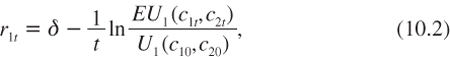
where U_i (c₁, c₂) is the partial derivative of U with respect to c_i. This economic discount rate allows the value of different consumption increments at different dates to be compared.

Consider alternatively an investment project that increases the environmental quality by ε at date t. The standard way to include this environmental impact in the cost-benefit analysis would be to first express this impact in future monetary terms. The instantaneous value v_t of the environment at date t is measured by the marginal rate of substitution between consumption and the environment:

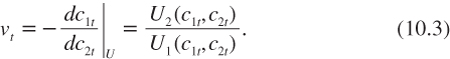
If the quality of the environment was tradable, v_t would be its equilibrium price, taking the aggregate consumption good as the numeraire. More generally, v_t is the instantaneous willingness to pay for a one-unit improvement in environmental quality. Its evolution over time is uncertain, so that seen from t = 0, v_t is a random variable, as is the future monetary benefit εv_t of the sure improvement in environmental quality. This implies that in spite of the fact that an investment project with a sure ecological benefit is being considered, its monetary benefit is uncertain. Up to now, this book has focused on the valuation of sure cash flows; extending the analysis to the valuation of uncertain projects will be carried out later in this book.

A much simpler approach is to define an ecological discount rate. Consider a marginal project that would increase environmental quality by a sure amount ε at date t, but would reduce the environmental quality by ε exp(–rt) today. Implementing this project would be socially efficient if

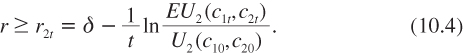
This equation defines the ecological discount rate r_2t for the time horizon t. It allows the comparison of sure changes in environmental quality at different dates. In particular, an increase in environmental quality by ε at date t has an effect on intertemporal welfare that is equivalent to an increase in current environmental quality by ε exp(–r_2tt). In monetary terms, this is equal to v₀ε exp(–r_2tt), where v₀ is the current value of one unit of environmental quality.

To sum up, the benefit of a unit increment in environmental quality at date t should be accounted for in the evaluation of a project as equivalent to an immediate increase in consumption by v₀ε exp(–r_2tt). This really means that environmental costs and benefits should be discounted at the ecological rate r_2t, which does not have to be the same as the economic discount rate r_1t. The potential discrepancy between the economic discount rate and the ecological discount rate takes into account the stochastic changes in the relative social valuation of the environment.

DETERMINANTS OF THE ECOLOGICAL DISCOUNT RATE

In this section, we examine the determinants of the rate r_2t with which a sure increase in environmental quality at date t should be discounted. It is characterized by equation (10.4). Let us first focus on the role of the level of c_2t and the uncertainty surrounding it. A better environmental quality in the future raises the ecological discount rate, ceteris paribus, because U is concave in c₂. This effect is symmetric to the wealth effect presented in chapter 2. One is ready to sacrifice less today if the future quality of the environment is larger because of the decreasing marginal utility of environmental quality. This is referred to as “the ecological growth effect.”

If it is assumed that U₂ is convex in c₂, then the uncertainty surrounding c_2t reduces the ecological discount rate. This effect, referred to as the “ecological prudence effect,” is analogous to the precautionary effect for monetary cash flows described in chapter 3. The basic idea is that one should do more to improve future environmental quality if it is more uncertain.

It is also necessary to take into account changes in GDP per capita, c_1t, on the level of the ecological discount rate. Suppose for example that the two goods are substitutes, which requires that the marginal utility of c₂ is decreasing in c₁. In other words, suppose that U₁₂ is negative. Then, an increase in the GDP per capita at date t reduces the marginal utility of environmental quality at that date. Therefore, it raises the ecological discount rate. This is referred to as “the substitution effect.”

One difficulty is to determine whether consumption and the environment are substitutes (U₁₂ ≤ 0) or complements (U₁₂ ≥ 0). Fortunately, there is a simple way to answer this question. Consider an arbitrary situation characterized by (c₁, c₂), an arbitrary reduction in consumption l₁ > 0, and an arbitrary reduction in environmental quality l₂ > 0. Consider two lotteries. Lottery A is a fifty-fifty chance of facing the monetary loss or the environmental loss. Lottery B is a fifty-fifty chance of facing the two losses simultaneously, or to lose nothing. If one prefers A to B, it must be that U₁₂ is negative. Indeed, it means that:

which is equivalent to:

This requires that U₁₂ is negative, or U is supermodular. Richard (1975), Epstein and Tanny (1980), Bommier (2007), and Eeckhoudt, Rey, and Schlesinger (2007) analyze this idea of “correlation aversion,” which is another way to say that the two goods are substitutes.

A more complex problem is to evaluate the effect of uncertainty about economic growth on the ecological discount rate. Obviously, a zero-mean risk on c_1t raises EU₂(c_1t, c_2t) if U₂ is convex in its first argument. This effect is referred to as the “cross-prudence in consumption” effect. In order to evaluate whether condition U₂₁₁≥ 0 is reasonable, the approach of Eeckhoudt et al. (2007) can be followed. They use a multidimensional version of equation (3.12), and again consider an arbitrary initial situation (c₁, c₂), an arbitrary zero-mean risk in consumption ε₁, and an arbitrary reduction in environmental quality l₂ > 0. Consider two lotteries. Lottery A is a fifty-fifty chance to face the monetary risk or the environmental loss. Lottery B is a fifty-fifty chance to face the monetary risk and the environmental loss simultaneously, or to lose nothing. If one prefers A to B, it must be that U₂₁₁ is positive. Indeed, this preference implies that:

which is equivalent to:

This requires that U₂ is convex in c₁. The preference of lottery A over lottery B provides an economic justification to reduce the ecological discount rate when the economic growth rate becomes more uncertain.

Finally, the existence of a positive correlation between economic growth and improvement in environmental quality provides a last determinant of the ecological discount rate. As many readers may now anticipate, this is formalized by a positive statistical dependence of (c_1t, c_2t) through the notion of an increase in concordance. Using lemma 2 of chapter 8, an increase in concordance raises EU₂(c_1t, c_2t) if and only if U₂ is supermodular, that is, if U₂₂₁ is positive. By symmetry to the notion of cross-prudence in consumption, this means that the representative agent is cross-prudent toward the environment. They prefer a lottery with a fifty-fifty chance to face either a sure monetary loss or a zero-mean environmental risk in isolation rather than a lottery with a fifty-fifty chance of facing both together or facing no risk at all. Under this assumption, the existence of a positive correlation in the economic and ecological growth rates raises EU₂(c_1t, c_2t), thereby reducing the efficient ecological discount rate. Intuitively, one wants to do more for the future when the economic and ecological risks are positively correlated than when they are independent. This is the “correlation effect.”

In this section, we assumed the sign of the cross-derivatives of the utility function to guarantee that the representative agent always prefers to incur one of the two harms for certain, with the only uncertainty being about which one will be received, as opposed to a 50-50 gamble of receiving the two harms simultaneously, or receiving neither. Following a terminology introduced by Eeckhoudt and Schlesinger (2006), pairs of harms are “mutually aggravating.”

Under this set of assumptions on U, the following factors raise the ecological discount rate:

• An increase in future environmental quality;

• An increase in future GDP per capita.

On the contrary, the following factors reduce it:

• An increase in the uncertainty affecting future environmental quality;

• An increase in the uncertainty affecting the future GDP per capita; and

• An increase in the correlation in the two risks.

A symmetric analysis can be made for the determinants of the economic discount rate r_1t.

AN ANALYTICAL SOLUTION

The integral EU₂(c_1t, c_2t) has an analytical solution in the special case of a bivariate geometric Brownian motion for (c_1t, c_2t) and a Cobb–Douglas utility function. Suppose that

in the domain (c₁,c₂)∈⁺². We suppose that

in order to guarantee that U is increasing in its two arguments. The concavity of U with respect to its two arguments requires that γ₁ and γ₂ are positive. If they are both larger than unity, it is easy to check that this utility function satisfies the assumptions made in the previous section that pairs of harms are “mutually aggravating,” that the two goods are substitutes, and that the agent is (cross-)prudent in consumption and in environmental quality:

In the same way as the benchmark univariate model presented in chapter 3, let us assume that (ln c_1t, ln c_2t) is normally distributed with mean (ln c₁₀+ µ₁t, ln c₂₀+ µ₂t) and variance-covariance matrix Σ = (σ_ij t)_{i,j = 1,2}. We have that:

where z_t = (1 –γ₁) ln c_1t – γ₂ ln c_2t is normally distributed with mean:

and variance:

Using lemma 1 yields:

By equation (10.4), we obtain that:

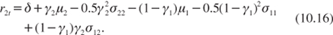
Finally, let g_i = t^-1 In (Ec_it/c_i0) = μ_i + 0.5σ_ii be the growth rate of Ec_it. Equation (10.16) can thus be rewritten as:

The term structure of the ecological discount rate is flat. In such an economy, the random evolution of aggregate consumption and environmental quality does not justify the use of a smaller discount rate for benefits occurring in a more distant future.

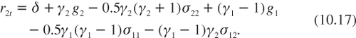
In addition to the rate of pure time preference, the five determinants of the ecological discount rate that were described in the previous section can be recognized in the right-hand side of equality (10.17):

• γ₂g₂ is the positive ecological growth effect, assuming an improving environmental quality;

• –0.5γ₂(γ₂ + 1)σ₂₂ is the negative ecological prudence effect;

• (γ₂ – 1)g₁ is the positive substitution effect, assuming a growing economy;

• –0.5γ₁(γ₁ – 1)σ₁₁ is the negative cross-prudence in consumption effect;

• –(γ₁ – 1)γ₂σ_γ is the negative correlation effect, assuming a positive correlation between the economic and ecological growth rates.

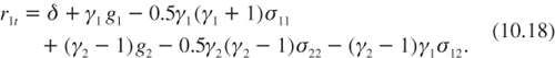
Symmetrically, we can compute the economic discount rate:

We can also determine the difference between the two discount rates:

Interestingly, under certainty, the difference between the two discount rates is independent of the parameters of the Cobb–Douglas utility function. This equation provides two arguments in favor of using an ecological discount rate that is smaller than the economic discount rate. First, it is often suggested that the growth rate for environmental quality is smaller than the economic growth rate (g₂ < g₁). Indeed, g₂ is potentially negative. Second, it seems that there is more uncertainty surrounding the evolution of environmental quality than the evolution of the economy itself (σ₂₂ > σ₁₁). If the degrees of aversion to risk on c₁ and on c₂ are not too heterogeneous, this implies that (γ₁σ₁₁ – γ₂σ₂₂ is negative. The last term on the right-hand side of equation (10.19) is more difficult to sign.

A CALIBRATION EXERCISE

Because of the lack of time-series data about environmental quality, calibrating the previous specification is problematic. Various authors have argued in favor of a closer link between environmental quality and economic growth. Following this idea, let us make the alternative assumption that the environmental quality is a deterministic function of economic achievement: c_2t = f(c_1t). Common wisdom suggests that environmental quality is a decreasing function of GDP per capita, but this is heavily debated in scientific circles. The environmental Kuznets curve hypothesis speculates that the relationship between per capita income and environmental quality has an inverted U-shape, but there is no consensus about the validity of this hypothesis (see for example Millimet, List, and Stengos 2003). From now on it is hypothesized that there is a monotone relationship by assuming that there exists ρ∈ such that where ρ can be either positive or negative. If we assume that c_1t follows a geometric Brownian motion, c_2t also follows a geometric Brownian motion, so that an analytical solution for the discount rates can be obtained. Using the standard trick of lemma 1, it follows that:

and

The interested reader can recover from these equations the different determinants of these two rates that were discussed earlier in the chapter.

In order to calibrate this model, let us assume that the rate of pure preference for the present δ is zero. It is also assumed, as before, that the relative aversion to risk on consumption is a constant γ₁ = 2. The parameter γ₂ for aversion to environmental risk is not easy to calibrate. Observe, however, that, if it were a tradable good, the share of total consumption expenditures that would be made up of expenditures on environmental quality is:

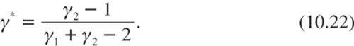
Hoel and Sterner (2007) and Sterner and Persson (2008) suggested γ^* somewhere between 10% and 50%, which implies that γ₂ should be somewhere between 1.1 and 2 under our specification. We hereafter assume γ^* = 0.3, which implies that γ₂ = 1.4. Suppose also that g₁ = 2%, and

The last parameter to calibrate is the elasticity ρ of environmental quality to changes in GDP per capita. The calibration depends upon how environmental quality is defined. In order to estimate ρ, the SYS_LAN indicator contained in the Environmental Sustainability Index (ESI2005, Yale Center for Environmental Law and Policy 2005) has been used. It measures, for 146 countries in 2005, the percentage of total land area (including inland waters) having very high anthropogenic impact. Let c₁ be the 2005 GDP per capita from the World Economic Outlook Database of IMF (April 2008), and c₂ be defined as 3 + SYS_LAN from ESI2005. In figure 10.1, we have represented this database and the associated OLS regression line, which is

The t-statistic for the slope-coefficient is –4.69, whereas the R2 coefficient equals 0.13. Plugging ρ = –0.10 in equations (10.20) and (10.21) yields

It is useful to provide a few comments on this result. First, the difference between the ecological rate and the economic rate comes mostly from the large expected economic growth rate (g₁ = 2%) compared to the expected environmental growth rate (g₂ = ρg₁ = –0.2%). Second, the level of the ecological discount rate is mostly determined by the substitution effect. Because ρ is small in absolute value, the (negative) ecological growth effect γ₂ρg₁ = –0.28% is also small, particularly in comparison to the substitution effect (γ₁-1)g₁ = 2%. Third, the effect of uncertainty (prudence, cross-prudence, and correlation effects) is marginal because of the low volatility of c₁ and c₂, and because it is assumed that shocks are not serially correlated. Finally, a comparison should be made between the economic discount rate obtained here and the one that was estimated at around 3.6% in chapter 3 (in the absence of separate treatment of environmental quality). Diminishing expectations about the quality of the environment and the associated substitution effect, (γ₂-1)ρg₁ = –0.08%, explains most of the discrepancy between the benchmark 3.6% and the 3.5% obtained here.

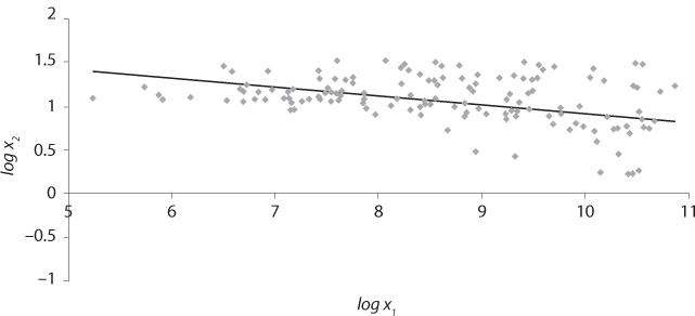
Figure 10.1. OLS regression using a panel of 146 countries in 2005, with c₁ being the GDP/cap (World Economic Outlook Database of IMF), and c₂ = 3 + SYS _ LAN (Environmental Sustainability Index 2005).

EXTENSION TO PARAMETRIC UNCERTAINTY

In the previous two specifications of the bivariate model, a geometric Brownian motion with known parameters was heavily relied upon. Without surprise, flat term structures were obtained under this framework. One easy extension can be made by recognizing that some of the parameters governing the stochastic economic and ecological growth are uncertain. Consider for example the model that we calibrated in the previous section, and suppose that the parameters (g₁, σ₁₁, ρ) depend upon a variable θ that is not known with certainty. Suppose as in chapter 6 that θ can take integer values 1 to n, respectively, with probabilities q₁, …, q_n. Then, as before, it is easy to derive from equation (10.4) that

where r₂(θ) is the ecological discount rate that would prevail if the true value of the unknown parameter would be θ, i.e.,

The reader is now accustomed to the fact that this model yields a decreasing term structure that converges to the smallest r₂(θ). A symmetric result holds for the economic discount rate.

Suppose for example that g₁ and σ₁₁ are known, but the elasticity ρ of environmental quality to changes in GDP is not. Rather than assuming that ρ = –0.1, as was estimated in the previous section (with a small R2 for the OLS estimation), let us suppose that ρ is either –0.6 or +0.4 with equal probabilities. All other parameters remain unchanged compared to the previous section. We draw the term structure of r_1t and r_2t in the next figure. Since the economic growth follows a Brownian motion, the economic discount rate is almost independent of the time horizon. It reduces to a lower rate of 3.2% for distant cash flows, which would be the efficient economic discount rate if the elasticity ρ was –0.6. In that case, the negative substitution effect would be stronger than in the benchmark case with ρ = –0.1. The ecological discount rate goes from 1.6% to 0.3% when t goes from 0 to infinity, as shown in figure 10.2. The high uncertainty affecting the long-term evolution of the environment in this specification explains why the term structure of the ecological discount rate is decreasing. Another way to interpret this result is obtained by examining the worst-case scenario. In the case in which ρ would be –0.6, the large economic growth rate would have a strong negative impact on the quality of the environment. This would generate a strong negative ecological growth effect, γ₂ρg₁ = –1.68%, which offsets most of the substitution effect (γ₁ – 1)g₁ = 2%.

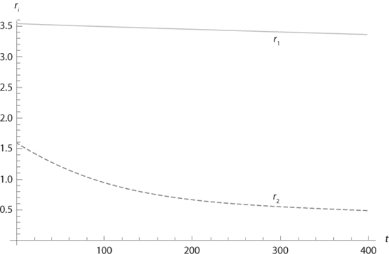
Figure 10.2. The economic and ecological discount rates with , δ = 0%, g₁ = 2%, and c_2t = c_1t with ρ ~ (–0.6, 1.2; 0.4, 1/2).

CES UTILITY FUNCTIONS

Guesnerie (2004), Hoel and Sterner (2007), Sterner and Persson (2008), and Traeger (2007) consider the case of certainty, which implies that the only determinants at play for the ecological discount rate are the ecological growth effect and the substitution effect. In exchange for this simplification, they examined a family of utility functions that are more general than the Cobb–Douglas specification. In particular, they assumed that U has constant elasticity of substitution σ > 0:

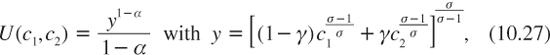
where α > 0 is relative aversion toward the risk on “aggregate good” y, and γ ∈ [0,1] is a preference weight in favor of the environment. Parameter σ is the percentage rate at which the demand for c₂ declines when the relative price of c₂ is increased by 1%. When s tends to unity, y tends to so that the Cobb–Douglas specification is obtained as a special case. When σ ≠ 1, the additive nature in y implies that it can never be lognormally distributed, thereby prohibiting the possibility of finding an analytical solution under uncertainty. We have that

It can be checked that the two goods are substitutes if ασ – 1 is positive. Under this condition, an increase in economic growth raises the ecological discount rate. Under the same condition, U₂₂ is negative, so that an anticipated deterioration in the quality of the environment reduces the ecological discount rate. To make this more explicit, suppose that growth rates are constant, which means that c_it = exp(g_it). The following equation is a direct rewriting of equation (10.4) under this specification:

with:

Observe that exp G(t) is the certainty equivalent of (exp g₁, 1–γ; exp g₂, γ) under utility function , it is increasing, and has an Arrow–Pratt coefficient of risk aversion which is increasing (decreasing) in t when σ is smaller (larger) than unity. This implies that the certainty equivalent G(t) is decreasing (increasing) in t when σ is smaller (larger) than unity. This implies in turn that the term structure of the ecological discount rate is decreasing if (ασ – 1)(1 – σ) is positive. More details are given in Guesnerie (2004), Guéant, Guesnerie, and Lasry (2009), and Gollier (2010).

SUMMARY OF MAIN RESULTS

1.  Most investment projects have economic and environmental impacts. Under the standard cost-benefit analysis, future environmental impacts are monetarized and discounted at the rate examined earlier in this book.

2.  An alternative approach consists in discounting future environmental impacts into present equivalent environmental impact, and to transform them into current monetary value. This ecological discount rate need not be equal to the rate at which economic impacts are discounted.

3.  The model examined in this chapter has a bivariate utility function. The standard marginalist approach allows us to derive two extended Ramsey rules respectively for the economic discount rate and for the ecological discount rate. In parallel to the wealth effect for the economic rate, there is an “ecological growth effect” which has a positive impact on the ecological rate if the environment improves over time and agents are averse to environmental inequalities.

4.  The two Ramsey rules have six terms. For the ecological rate, we have impatience, the aversion to inequality with respect to the environment, the prudence toward environmental risks, in addition to three other terms linked to the interactions between economic and environmental elements in the utility function. One of them is a substitution effect. If the two goods are substitutes, the economic growth reduces the future value of the environment, thereby raising the ecological rate.

REFERENCES

Bommier, A. (2007), Risk aversion, intertemporal elasticity of substitution and correlation aversion, Economics Bulletin, 29, 1–8.

Cropper, M. L., S. K. Aydede, and P. R. Portney (1994), Public preferences for life saving: discounting for time and age, Journal of Risk and Uncertainty, 8, 243–265.

Cropper, M. L., J. K. Hammitt, and L. A. Robinson (2011), Valuing Mortality-Risk Reductions: Progress and Challenges, Annual Review of Resource Economics, in press (also published as National Bureau of Economic Research Working Paper 16971, April 2011).

Cropper, M. L., and P. R. Portney (1990), Discounting and the evaluation of life-saving programs, Journal of Risk and Uncertainty, 3, 369–379.

Eeckhoudt, L., B. Rey, and H. Schlesinger (2007), A good sign for multivariate risk taking, Management Science, 53 (1), 117–124.

Eeckhoudt, L., and H. Schlesinger (2006), Putting risk in its proper place, American Economic Review, 96(1), 280–289.

Epstein, L. G., and S. M. Tanny (1980), Increasing generalized correlation: a definition and some economic consequences, Canadian Journal of Economics, 13, 16–34.

Gollier, C. (2010), Ecological discounting, Journal of Economic Theory, 145, 812–829.

Guéant, O., R. Guesnerie, and J.-M. Lasry (2009), Ecological intuition versus economic “reason,” mimeo, Paris School of Economics.

Guesnerie, R. (2004), Calcul économique et développement durable, Revue Economique, 55, 363–382.

Hoel, M., and T. Sterner (2007), Discounting and relative prices, Climatic Change, DOI 10.1007/s10584-007-9255-2, March 2007.

Malinvaud, E. (1953), Capital accumulation and efficient allocation of resources, Econometrica, 21 (2), 233–268.

Millimet, D. L., J. A. List, and T. Stengos (2003), The environmental Kuznets curve: Real progress or misspecified models? Review of Economics and Statistics, 85, 1038–1047.

Richard, S. F. (1975), Multivariate risk aversion, utility independence and separable utility functions, Management Science, 22, 12–21.

Sterner, T., and M. Persson (2008), An Even Sterner Report: Introducing relative prices into the discounting debate, Review of Environmental Economics and Policy, 2 (1), 61–76.

Traeger, C. P. (2007), Sustainability, limited substitutability and non-constant social discount rates, Department of Agricultural & Resource Economics DP 1045, Berkeley.

Weikard, H.-P., and X. Zhu (2005), Discounting and environmental quality: When should dual rates be used? Economic Modelling, 22, 868–878.

Yale Center for Environmental Law and Policy (2005), 2005 Environmental Sustainability Index: Benchmarking national environmental stewardship, Yale University.