
Chapter 5
Modeling for Product Release Planning
5.1 Introduction
Modeling is an art. It is the art of describing essential parts of reality for the purpose of its further analysis. Depending on what we hope to achieve and also depending on the data and information available, the models will be more or less detailed.
The mere formulation of a problem is far more essential than its solution, which may be merely a matter of mathematical or experimental skills. To raise new questions (and), new possibilities, to regard old problems from a new angle, requires creative imagination and marks real advances in science.
Models in general are abstract and simplified descriptions of reality. According to the objectives and the specific topic under investigation, models are always focusing on specific aspects of reality. Many concerns have to be left out to keep the model tractable. In the cases where reality is dynamically changing, models have to be adapted correspondingly.
This chapter is devoted to modeling for the purpose of product release planning. The decision about the level of detail of the model is important. Its answer depends on the scope of the planning and the level of detail expected from the planning results. As expectations from planning are varying, there is no one size fits all type of model. Instead, the content, size and granularity of the model are context specific.
In this chapter, different components of release planning models are studied. A variety of modeling options is presented. As a result, the readers will have different possibilities to find the most appropriate model components, applicable for their specific purposes. This model is then used as an input for Chapter 6 when utilized for planning.
5.2 Decision Variables and Horizon of Planning
Decisions in product release planning are primarily related to features and their assignment to releases. Consequently, decision variables are related to a set of features under consideration. Let F = {f(1),.. .,f(N)} be a set of candidate features. At this point, the assumption is that the features are known and are well described. Their (given) description is used to prioritize them.
It needs to be specified how far in advance planning should be done. This is the number of product releases to consider for planning purposes. Our model allows us to go beyond just looking at the next release. In general, K releases of the product are considered. In case of K equal to one, planning is just for the next release.
Even though the degree of uncertainty grows for each later release, it is often useful to have a more long-term perspective. Customers want an answer regarding when a specific feature is planned to be provided. This information is closely related to the competitiveness of the product. If a company is able to provide key features ahead of their competitors, then this is attractive from a sales and marketing point of view. In addition, the release plan of a product also provides guidance for the development team on the sequence of features to be implemented.
The decision variables x(n) (n = 1...N) describing the proposed strategy for handling features f(n) provide answers to two questions:
Is feature f(n) part of any of the next K product releases?
If yes, at which release is the feature f(n) offered?
Each individual release plan x describes the assignment to releases for all candidate features. It is characterized by a vector x = (x(1),...,x(N)) defined by (5.1) and (5.2).
(5.1) |
x(n) = k |
if feature f(n) is offered at release k (n = 1…N) |
(5.2) |
x(n) = K+1 |
if feature f(n) is postponed, i.e., it is not offered in one of the next K product releases (n = 1…N) |
5.3 Dependencies Between Features
A number of additional constraints need to be considered for the decision about features and their assignment to releases. From analyzing industrial software product release planning projects in the domain of telecommunications, [Carlshamre et al. ‘01] observed that features are often dependent on each other. For the projects and the domain analyzed, the percentage of features being dependent in one way or the other was as high as 80%.
There is a variety of types of dependencies. In [Carlshamre et al. ‘01], six different types were analyzed. In what follows, a list of eight types of dependencies is presented in more detail. The term dependency here can mean different things. It can be related to dependencies in the
Implementation space (two features are “close” in their implementation and should be treated together), or
Feature effort space (two features are impacting each other in their implementation effort if provided in the same release), or
Feature value space (two features are impacting each other in their value if provided in the same release), and
Feature usage space (two features are only useful for the user if provided in the same release).
Feature dependencies can be visualized by a feature dependency graph. The vertices of the graph correspond to the features, and the arcs (directed connection between vertices) and edges (undirected connections between vertices) correspond to one of the different types of dependencies illustrated in Figure 5.1.
5.3.1 Type 1: Coupling
Feature A is coupled to feature B means that both features should be offered in the same release. The reason for this is that both features depend on each other. For a text processing system, the user would expect the feature Copy and the feature Paste to be in the same release. Alternatively, the coupling relationship can also be based on another form of dependency such as the closeness in the implementation of the features, that is, whenever one of the features is implemented, the other one should be implemented as well.
5.3.2 Type 2: Either or
Features A and B are in an either or dependency relationship if exactly one of them needs to be taken. That means, if A is selected then B cannot be selected and vice versa. Selection here means that the feature is offered in one of the product releases under consideration.
5.3.3 Type 3: At least one
For a set of features A, B, C ... the at least one dependency means that among the features, at least one should be selected for one of the releases in consideration. Consequently, choosing none of the features would violate this dependency condition, while choosing more than one would not.
5.3.4 Type 4: At most one
For a set of features A, B, C ... the at most one dependency means that among the features, at most one should be selected for one of the releases in consideration. Consequently, choosing more than one of the features would violate this dependency condition, while choosing none of them would not.
5.3.5 Type 5: Weak precedence
Features A and B are in a weak precedence dependency (A weakly precedes B) if feature A cannot be offered in release later than feature B. However, feature A can be offered in the same release as feature B.

Figure 5.1 Types of features dependencies and their visualization
5.3.6 Type 6: Strict precedence
Feature A and B are in a strict precedence dependency (A strictly precedes B) if feature A has to be offered at an earlier release than feature B. In the strict precedence relationship, both features cannot be offered in the same release.
5.3.7 Type 7: Value dependency
A set of features A, B, C ... are in a value dependency if the features are offered together in the same release, and the value of the features in conjunction exceeds the value from taking the sum of all the single values. Value dependency offers a bonus in the case that a certain number of features are offered in conjunction.
5.3.8 Type 8: Effort dependency
A set of features A, B, C ... is in an effort dependency if the features are offered together in the same release, and the total effort of the features is less than the effort from taking the sum of all the single values. Effort dependency is motivated by possible synergies between features when they are implemented in the same release.
5.4 Pre-Assignments
5.4.1 Overview
Pre-assignment of a feature to specific release is one possibility of enlarging the modeling options for the human user. The general purpose of release planning is to assign features to releases. For making this decision, the (subjective) priorities assigned to features by the different stakeholders and the (estimated) amount of resources consumed by the features are taken into account. Both types of information are geared toward making a largely objective decision.
Independent of the method selected for fact-based planning, there might be situations and scenarios where the assignment of features to releases is prescribed. These situations can be related to important legal constraints, aspects of competitiveness (a feature should not be released later than a given release), or (non-) availability of resources. In other words, pre-assignment makes the human decision (assigning a feature to a release) more important than what any computer-supported planning method is proposing.
Pre-assignment can be done in two principal ways. First, a feature can be prescribed to be assigned in exactly one specific release. Second, a feature can be prescribed to be assigned in an interval (sequence) of releases. In both cases, the intention is to overwrite any other considerations executed by the planning system (trying to optimize in the range of flexibility available).
For planning K releases ahead, three options for pre-assignment of features are considered:
5.4.2 Option 1: Fixed pre-assignment of a feature to release k
Option 1 means that the feature needs to be released in fixed release k where k is any of the possible releases 1... K+1. This convention is used to say that a feature is pre-assigned to release K+1 if it is requested to be postponed.
5.4.3 Option 2: Pre-assignment of a feature not later than release k
Option 2 means that the feature needs to be released no later than at release k where k is one out of the possible releases from 2 to K. For release K this implies that the feature cannot be postponed.
5.4.4 Option 3: Pre-assignment of a feature not earlier than release k
Option 3 means that the feature needs to be released no earlier than at release k where k is one out of the possible releases from 2 to K.
5.4.5 Illustration
The three different options for pre-assignment are illustrated in Figure 5.2. In the case of planning K = 4 releases ahead of time, the points in the grid indicate the possible assignments of features to releases. For example, if there is a pre-assignment not later than release 3 for a feature, then this feature can be assigned to one of the releases 1, 2 or 3. This is shown in the second row of Figure 5.2. As another example, a feature can be pre-assigned to a fixed release (as shown for the top row for the assignment to release 2).
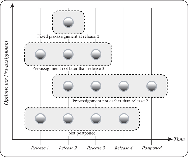
Figure 5.2 Four example options for pre-assignment of features to releases
5.5 Effort Constraints
Planning without investigating the resource constraints is risky, as the resulting plans are likely to fail because of the potential lack of sufficient resources for the implementation of the features. In its simplest form, a variable called effort is introduced, which subsumes the estimated effort needed to implement a feature. The effort for implementing feature f(n) is denoted by effort(n). It can be measured in person days or, more fine-grained, in person hours. Later in this chapter, the total effort is further differentiated according to the different roles, tools and life-cycle phases involved in feature implementation.
When planning for K subsequent releases, the consumed effort per release is not allowed to exceed a given release capacity. For release k = 1...K, this capacity is denoted by Cap(k). More formally, a feasible release plan x needs to satisfy all the constraints
(5.3) Σn: x(n)=k effort(n) ≤ Cap(k) for k = 1…K
In (5.3), for each release k, the summation is taken over all features f(n) assigned to this release.
5.6 Cost Constraints
Similar to the effort constraints as just formulated, cost constraints can be introduced. In this case, each feature f(n) is consuming a certain amount of cost denoted by cost(n). This cost estimate subsumes all the different types of resource consumptions including human and non-human constraints. The different hourly rates of human resources are then aggregated into one cost measure per feature.
Using Budget(k) for the maximum amount of cost available for release k, the corresponding cost constraints are then formulated as
(5.4) Σn: x(n)=k cost(n) ≤ Budget(k) for k = 1…K
5.7 Resource Constraints
5.7.1 Overview
Just looking into cost or effort is a first approximation of describing the resources necessary for implementation of features. This first approximation does not consider individual types of resources. In this chapter, all key resources necessary for performing the tasks assigned to this release are considered. At strategic level, only cumulative consumption per release is considered for the different resources. At a more operational level, a time-dependent allocation of human and other resources to individual tasks creating the features have to be taken into account.
The estimated consumption of resources by features is considered part of the modeling effort. Different methods are applicable for providing estimates. Most of these methods incorporate some form of learning from former projects. In addition, often these methods are hybrid in the sense that they combine formal techniques with the judgment and expertise of human domain experts. For an overview of resource estimation methods, refer to [Briand and Wieczorek ‘02]. For a method of hybrid estimation specific to release planning called AQUA-RP, see Section 9.2.
The definition of the actual resource types is project-specific and is done by the product manager (in collaboration with the project manager). Resources can be defined in correspondence of the product life-cycle role (for example, design, implementation, testing) or related to specific skills (for example, user interface implementation, back-end algorithms in C++).
While the granularity in the consideration of resources is flexible, the actual number of resources needs to be selected with care. The planning problem gets more complicated if more resources are involved. Often, it is well known which resources are critical for the project because they became the bottleneck in former projects. These ones are the first candidates to look at in planning.
Independent of the content of the resources, there are two different types of resources to be considered in planning. They are called local respectively global in correspondence to their mode of spending.
Definition (Local resource): A resource is called local if the feature-related consumption of the resource is limited to exactly the release in which the feature is offered. Resources of this class are called local based on their spending mode. C
Definition (Global resource): A resource is called global if the feature-related consumption of the resource can be distributed across different release periods. C
All types of human resources that are available only for a specific release period are in the category of local resources. Global resources can be spent whenever there is capacity left over. This means that there is no request to use this resource in the specific release where it is finally offered. In what follows, the constraints related to the two resource types are discussed separately.
5.7.2 Constraints for local resources
When planning for R different resource types and K releases ahead of time, each proposed product release plan needs to fulfill R-K resource constraints. The constraints for each release are formulated separately, starting with the first release. Per release and in each of the R constraints, the summation is taken over all the features f(n) assigned to the first release.
For a given plan x and all types r (r = 1...R) of resources, the total consumption called Consumption (k,r,x) within release period k is not allowed to exceed the respective capacity called Capacity(k,r). The variable consumption(n,r) denotes the (estimated) consumption of resource type r by feature f(n). More specifically, the following constraints need to be satisfied for the R resource types in release period 1:
(5.5) Consumption(1,1,x) = Σn:x(n)=1 consumption(n,1) ≤ Capacity(1,1)
Consumption(1,2,x) = Σn:x(n)=1 consumption(n,2) ≤ Capacity(1,2)
...
Consumption(1,R,x) = Σn: x(n)=1 consumption(n,R) ≤ Capacity(1,R)
In the same way, the constraints for all subsequent releases k=2.. .K are formulated. Now, summation is done for all features f(n) which are assigned to a fixed release k (k = 2...K):
(5.6) ΣConsumption(k,1,x) = Σn: x(n)=k consumption(n,1) ≤ Capacity(k,1)
Consumption(k,2,x) = Σn: x(n)=k consumption(n,2) ≤ Capacity(k,2)
...
Consumption(k,R,x) = Σn: x(n)=k consumption(n,R) ≤ Capacity(k,R)
5.7.3 Constraints for global resources
Resource constraints for global resources look different from those of local resources. Their formulation is given in (5.7) to (5.9). The difference to the former (local resource type) constraints is the fact that when considering a release period k, all features not yet released before k potentially can be worked on. This implies the need for a three-dimensional matrix denoted by Percentagex, which is used to describe how implementation of the features is organized for a given release plan x. The values Percentagex(n,k,r) describe the percentage of spending in release k for resource type r when looking at feature f(n).
(5.7) Σn =1..N Percentagex(n,k,1) consumption(n,1) ≤ Capacity(k,1) for all releases k = 1…K
Σn=1..N Percentagex(n,k,2) consumption(n,2) ≤ Capacity(k,2) for all releases k = 1…K.
Σn=1..N Percentagex(n,k,R) consumption(n,R) ≤ Capacity(k,R) for all releases k = 1…K(5.8) 0 ≤ Percentagex(n,k,r) ≤ 1 for all resources r = 1…R, for all releases k = 1…K, and for all features f(n), n = 1…N
In addition to all the constraints formulated per releases, it needs to be ensured that the total of all consumptions for feature f(n) across releases equals the total demand of resource r per feature. This is illustrated in Figure 5.3. At the upper part, 100% of the resource consumption of features f(1), f(2) and f(3) is spent in exactly one release period. This is different at the lower part where the resource spending is allocated over different release periods. The related consumption constraint is formulated in (5.9).
(5.9) Σk = 1 .. K Percentagex(n,k,r) = 1 for all r = 1... R and for all n = 1…N
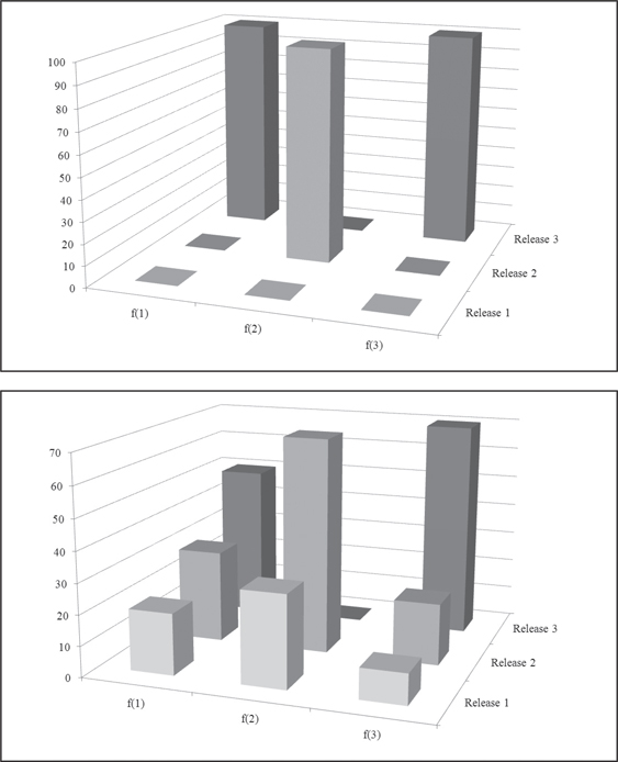
Figure 5.3 Comparison of consumption between local (top) and global (bottom) resource types
5.8 Risk Constraints
There are different types of risk associated with a feature. For example, there is the risk of implementation, the risk of acceptance, the risk of dependency from subcontractors and the risk of maintenance. Consideration of all these risks (and maybe others) is important. However, it is difficult to treat them in a quantitative manner as part of a systematic planning method.
Besides the classification and quantification of risk, it is not clear up-front what constitutes the right way to approach risk. As part of an incremental method, does it mean that as many as possible of the higher risks should be considered in earlier releases? Or vice versa, would it make more sense to postpone the risky features to later stages? Or is a balancing of the total amount of risk per release the recommended strategy?
A simplified modeling approach introduced is intended to influence release planning strategies by at least some consideration of risk. As part of that, a classification of (one selected type) risk into a five-point scale is done. The categories are called VERY LOW, LOW, AVERAGE, HIGH and VERY HIGH risk. Each feature is assigned to one of the five categories. Consequently, risk(n) = HIGH means that the feature f(n) is classified according to the specified risk as belonging to the HIGH risk category.
The term #(category, k) denotes the given bound for occurrence of features assigned to release phase k and being of the specific risk category under consideration. For example, #(VERY HIGH, 1) means the number of very high risk features allowed for release 1.
Using this notation, risk related constraints can be introduced by just limiting the number of risks of a specified category per releases. Ignoring Low and Very Low risk categories, the following constraints (5.10) − (5.12) are obtained.
(5.10) Σn:risk(n)=VERY HIGH 1 ≤ #(VERY HIGH, k) for k = 1…K
(5.11) Σn:risk(n)=HIGH 1 ≤ #(HIGH, k) for k = 1…K
(5.12) Σn:risk(n)=AVERAGE 1 ≤ #(AVERAGE, k) for k = 1…K
All release plans generated under one of these constraints would then satisfy the limit of risky features per release in each of the selected risk categories. The definition of the risk level is done by the product manager in consultation with the domain expert. It is largely based on former project and product experience.
5.9 Planning Objectives
5.9.1 Overview
Planning objectives give the orientation for deriving appropriate plans. Definition of the actual planning objectives is of key importance. There are a number of potential objectives, and their selection and proper balance needs careful consideration. The top-down approach for this selection starts with the strategic view of the company. From there, a projection to strategic or operational planning objectives is done. The whole process can be subdivided into three essential steps:
Definition of the most important planning objectives derived from business goals
Selection of the most relevant objectives for the actual product planning
Formalization (putting the informally stated objectives into a formalized planning function)
Business goals often vary over time and are company specific. In most cases, there is more than one objective to be pursued strategically. The Balanced Score Card method [Kaplan and Norton ‘92] is one prominent example for consideration of multiple objectives. The more specific, measurable and time-oriented the formulated goals are, the higher the chance of actually achieving them or adjusting the goals to changed conditions.
5.9.2 Candidate objectives for the evaluation of product release plans
Operational goals for requirements prioritization have been discussed by [Firesmith ‘04]. Most of them (listed in Section 3.5) can be extended to evaluation of product releases as well. “Good” plans are based on “good” features, but there are additional aspects related to how the features composed into one release fit together. The number of relevant criteria, the criteria themselves and the composition and weighting of the chosen criteria are very company and project specific and need to be decided based on a case-by-case analysis.
5.9.3 Stakeholder feature points
Besides the selection of planning objectives, another question is how to combine them. However, there is the additional problem of compatibility: How does one combine different criteria; for example, such criteria as the cost of implementation for a plan and the criterion of urgency of the features offered by a plan? One way to handle this problem is to provide scores to each plan for each criterion and to integrate all the scores into one overall utility value of the plan. This idea is implemented in the concept of stakeholder feature points.
Stakeholder feature points are a measure defined for each feature in conjunction with a release plan x. The measure describes the stakeholder satisfaction related to a plan x. The higher the number of stakeholder feature points, the higher the expected satisfaction of stakeholders with this plan.
The calculation of stakeholder feature points is based upon the scores of the stakeholder to features, the importance of the stakeholders, the importance of the criteria, and the importance of the different releases. In what follows, the key notation necessary for giving a formal definition of stakeholder feature points is introduced. The following parameters are used:
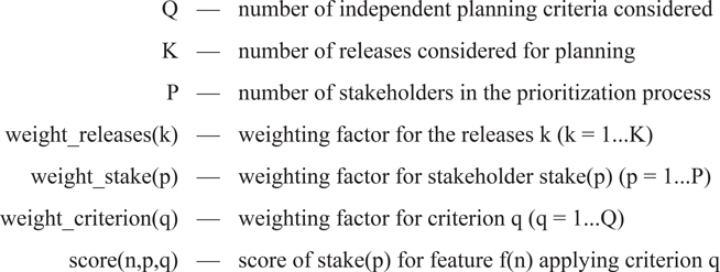
All of the weighting factors allow for the expression of relative degrees of importance. Although defined on an ordinal scale, later the weights will be treated like ratio scale measures. A pre-requisite for this interpretation is that their relative importance does not exceed one order of magnitude.
The prioritization process is the same as outlined in Chapter 3. The factors describing the level of importance for both stakeholders and criteria have already been introduced in Chapter 3 as part of the Multi-score method. The release weight factor weight_release(k) gives the relative importance of having a feature f(n) assigned to a release k. As a default, weightrelease (k) ≥ weight_release(k+1) for all k = 1... K-1. What that means is that the feature contribution to the overall objective is higher the earlier the feature is delivered.
Score(n,q) is the portion of the total number of stakeholder feature points, which is provided by feature f(n) when looked at criterion q. It is formally defined as the weighted sum (5.13) from all individual stakeholder scores on this criterion. In the case of stakeholders excluded for scoring on a given feature f(n), the calculation of Score(n,q) needs to be adjusted by just looking at the active stakeholders.
(5.13) Score(n,q) = Σ p = 1…P weight_stake(p)• score(n,p,q)
The variable SCORE(n) defined in (5.14) is based on all the individual contributions (5.13). It combines them in consideration of the degree of importance of the different criteria.
(5.14) SCORE(n) = Σ q = 1…Q weight_criterion(q)•Score(n,q)
Using (5.14) allows the definition of stakeholder feature points gained from plan x for feature f(n). The stakeholder feature points sfp(n,x) according to plan x are a measure describing the contribution of the feature f(n) to the overall utility of plan x. The number sfp(n,x) is defined in (5.15).
(5.15) sfp(n,x) = Σ k: x(n) = k weight_release(k)•SCORE(n)
If a feature is postponed, then it does not provide any stakeholder feature points. As stakeholder feature points are determined based on stakeholder scoring, their value correlates with the conformance between stakeholder priorities and the provision of features. The better the conformance per stakeholder, the higher the number sfp(n,x) of stakeholder feature points.
The objective of planning in this model is to maximize the total number of stakeholder feature points (TSFP). The process of calculating TSFP(x) is based upon the concrete data for features, stakeholders, prioritization criteria and releases. The steps of the process are illustrated in Figure 5.4. For a given plan x, the number TSFP(x) is defined in (5.16).
(5.16) TSFP (x) = Σ n = 1…N sfp(n,x)
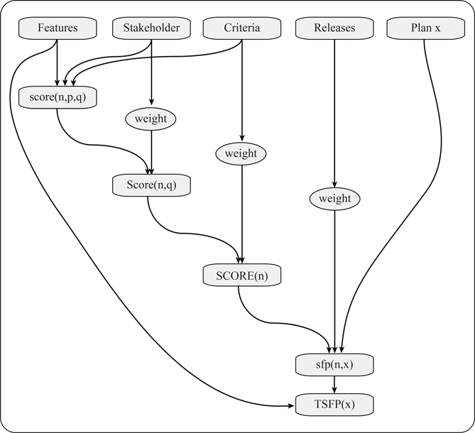
Figure 5.4 Calculation of total number of stakeholder feature points
The rationale for this function is that it reflects the objective of providing features of high stakeholder priority as early as possible. This is true the more important the stakeholder is considered. The underlying assumption is that stakeholder feature points are additive among the features, among the stakeholders and among the different criteria. The advantage of maximizing the total number of stakeholder feature points is that it is a compensational model, which allows linear combination of different criteria.
5.9.4 Non-linear objective functions
The assumption of additivity underlying the computation of TSFP(x) might not be applicable all the time, and other (non-linear) models can be considered as well. The actual composition of the planning function depends on the specific characteristics of the problem. Linear functions are easier to handle than non-linear ones.
However, in some cases it might be more appropriate to deviate from the linearity assumption. Some examples are given in (5.17) and (5.18). In these formulations, utility(n,k) denotes the overall utility obtained when feature f(n) is assigned to release option k. In (5.17), the results of scoring related to two criteria are multiplied. In (5.18), the minimum of the scoring results for three criteria is used for definition of overall utility of feature f(n) in release k.
(5.17) utility(n,k) = value(n,k) • urgency(n,k)
(5.18) utility(n,k) = Min {value(n,k), urgency(n,k), risk(n,k)}
In both cases, the different values are as weighted averages taken over all valid stakeholder priorities. While applied on a nine-point scale defined here, the Min operator and the product of values are applicable to other criteria as well.
5.9.5 Financial value maximization
The formulations (5.17) and (5.18), are still based on the compensatory model using stakeholder scores. Instead of relying on scoring of importance provided by the set of stakeholders, using one or the other form expressing the financial value of features is another alternative to formulate the objective of planning. In the spirit of value-based software engineering [Boehm and Huang ‘03], it is acknowledged that product development is a (financial) value creation process. What is needed for financially driven product release planning are appropriate measures to express the financial value.
The measure describing the financial value of a feature needs to be defined in dependence of time (which is the actual release date) and some assumed time horizon (which is the final release date). Consideration of time-dependent value functions in conjunction with flexible within some interval) release dates is further studied in [McElroy and Ruhe ‘10]. Another important consideration is that financial value is cumulative over time. Consequently, the earlier a feature is offered, the more time is available to create financial value out of this feature.
There are different financial measures that can be considered for this purpose. Two frequently used measures are:
Return on investment (ROI): For each point in time, the ROI expresses the ratio between the total profit made versus the total investment done for the period of time in consideration.
Net present value (NPV) gives the sum of the present values of features.
NPV assumes a given interest rate and a sequence of estimated cash flows starting from the defined release date. In this case, a feature is primarily judged based on its projected net present value assuming it will be offered at some release. This type of objective looks more accurate than stakeholder scores on a nine-point scale. However, value estimates are hard to get and uncertain in their nature.
5.10 Generation of Qualified Alternative Solutions
The traditional perspective of planning is to search for just one solution, which is qualified in some specific aspect. The quality of each solution is measured by a stated utility function. In our case, this means maximizing the total number of stakeholder points. A solution is called the best when there is no other solution performing better. There is a good chance that more than one best solution exists. Moreover, solutions close to the best possible ones might be of strong interest as well. The concept of K-best solutions and the diversification principle both aim at further analysis of solutions close to the best ones.
5.10.1 The diversification principle
The idea of looking for K-best solutions instead of just one was initially applied in [Murty ‘68] for generating solutions of the assignment problem. A solution set of cardinality K > 1 is generated with the property that there is no feasible solution outside this set with a better objective function value than any of the K-best solutions. Computation of K-best solutions has been done (among others) for the assignment problem [Lawler ‘72], the perfect matching problem [Chegireddy and Hamacher ‘85], and the traveling salesman problem [Van Der Poort et al. ‘99].
The principle of diversification goes beyond the calculation of the K-best solutions. It considers diversification between the solutions offered to be an essential asset. In certain situations, when the K-best solutions chosen are very similar, the advantage provided by the set of solutions is reduced. By observing that a more diversified set of solutions provides a richer understanding and a deeper insight of the problem, the principle of diversification is proposed.
Informally, a qualified alternative solution subsumes two different aspects of problem solving:
Qualified in the sense of solving the right problem. The proposed (qualified) release plan is assumed to be meaningful for the original (real-world) problem. This can be judged by a human expert having the capability to describe the problem and to evaluate a proposed solution.
Qualified in the sense of solving the problem right. The proposed (qualified) release plan is assumed to be of a guaranteed level of quality for the formalized problem. This can be achieved primarily by utilizing the strength and efficiency of computational algorithms.
Our key assumption for introducing diversification among a set of alternative solutions is as follows:
What this principle suggests is to work with an approximate model and compensate the (incomplete) model by considering a structurally diversified set of (qualified) solution alternatives that are proven to be close to the optimal solution. The role of this set of solutions is not limited to just providing a short list of candidate solutions. It can also provide more insight into the problem. Through the observation and comparison of different qualified solutions, one can gain important information about the inherent structure of the problem. For the example of release planning, if a feature is consistently assigned to the same release among all the candidate plans, this is a strong argument that this assignment is strongly suggested and that this assignment is quite robust.
5.10.2 Qualified solution alternatives
In what follows, some necessary definitions are provided in order to formulate the diversification principle more precisely. The maximization of the TSFP is considered again as the objective of planning.
(5.19) max {TSFP(x): x ∊ X}
In (5.19), X denotes a set of feasible release plans. A plan is called feasible if it fulfills all the explicitly stated constraints. The intension is to reduce the (typically large) size of the set of X based on a predefined target quality level α ∈ (0,1]. With the maximum objective function value TSFP* = max {TSFP(x): x ∈ X}, α-qualified solutions are defined as follows:
Definition (α-qualified solution): A solution x is called α-qualified if
(5.20) TSFP(x) ≥ α TSFP* and x ∊ X □
A given set of α-qualified (release plan) solutions is abbreviated by Xα. Once α is given, all solutions in Xα are considered to be as sufficiently good, and differences between solutions in Xα are considered to be insignificant. The justification for that consideration is the uncertainty of the available data as well as the uncertainty of the whole problem formulation. Often, the value of α is defined by α = 0.95 or α = 0.9.
5.10.3 Diversified solution alternatives
In order to increase the likelihood to solve the right problem, it is expect to provide a set of alternative solutions that is not only a-qualified, but also structurally diversified. For the purpose of characterization of the degree of diversification of the selected set of solutions, the notion of (structural) diversity is introduced. The classical way to model the diversity (or similarity, if interpretation is changed) between two solutions x1, x2 is to define a distance measure on the solution space. The distance measure is assumed to fulfill the properties of being reflexive (the solution to itself), symmetric (between two solutions) and transitive (between three solutions) [Arkhangelskii and Pontryagin ‘90].
One well-known distance measure is called Euclidean distance. Another example measure is the Hamming distance between two strings of equal length, defined as the number of positions for which the corresponding symbols are different [Hamming ‘50]. Once the distance between two solutions of a set is defined, the diversification of a set X of solutions can be computed as the sum of all the distances between all pairs of solutions in X.
Because an absolute measure is hard to evaluate independently of the context, a relative diversification measure is introduced instead. This normalized measure relates the actual distance to the maximum distance possible. From this relative measure it is easier to judge the degree of diversification being independent of the concrete context. See [Ngo-The and Ruhe ‘08] for further details.
5.11 How all the Modeling Components Come Together
In Sections 5.2 to 5.8, different options for technological, resource, cost and risk constraints have been described. For each individual problem, the actual set of constraints needs to be defined specifically. Sections 5.9 and 5.10 have offered different options for formulating the objective of planning. The differences are in the form of the planning function as well as in the final goal of the planning procedure (one single solution versus a solution set). At the end of this chapter, three formulations (called schemata) of the release planning problem are given. These formulations combine the definition of constraints provided in Sections 5.2 to 5.8 with the definition of the objective of planning given in Sections 5.9 and 5.10.
Release Planning Scheme RPP1
RPP1 looks for one final planning alternative. Given a set of feasible release plans X and a utility function Utility(x) defined on X. Among a set Xα of qualified and diversified planning alternatives, determine one final plan. The selection of this plan is done by human experts and is possibly based upon the potential match of the plan with some additional implicit concerns.
Release Planning Scheme RPP2
RPP2 looks for a set of qualified planning alternatives. Given a set X of feasible release plans and a utility function Utility(x) defined on X. Among all feasible planning alternatives, the problem is to determine a set of (five) qualified and diversified planning alternatives.
Release Planning Scheme RPP3
RRP3 looks for a set of trade-off solution alternatives. Given a set X of feasible release plans and two planning criteria formulated by functions G1(x) and G2(x) defined on X. Functions G1(x) and G2(x) are assumed to be maximized.
Looking for trade-off solutions means determining all plans x with the property that there is no other plan x’ fulfilling (5.21). What that means is that a plan x is a trade-off solution if there is no other plan that is better in one criterion and not worse in the other. Typically, there are several alternatives forming the set of tradeoff solutions.
(5.21) (G1(x’), G2(x’)) ≥ (G1(x), G2(x)) and
(G1(x’), G2(x’)) ≠ (G1(x), G2(x))
For example, in [Saliu and Ruhe ‘07], the trade-off between total feature value and ease of implementation of features was studied (see also Section 9.4). Among all feasible planning alternatives, the problem is to determine a set of trade-off solutions.
Solution method EVOLVE II looks at RPP1. For that purpose, RPP2 is used as an intermediate step. Formulation RPP3 is applied in Section 14.3 for the purpose of balancing between functional and non-functional requirements. One solution method for generating the trade-off curve is to introduce one of the two objectives as an additional constraint for solving the remaining one-criterion problem. From parametric variation of the constraint level, trade-off points can be obtained from application of the one-criterion solution method. For details on solution methods for multi-criteria optimization, see [Steuer ‘86].