In this chapter, we return to using mathematics. We’ve already covered addition, subtraction, and a collection of bit operations on our 64-bit registers. Now, we will learn multiplication and division.
We will program multiply with accumulate instructions. But first of all, we will provide some background on why the ARM processor has so much circuitry dedicated to performing this operation. This will get us into the mechanics of vector and matrix multiplication.
Multiplication
Xd is the lower 64 bits of the product. The upper 64 bits are discarded.
There is no “S” version of this instruction, so no condition flags can be set. Therefore, you can’t detect an overflow.
There aren’t separate signed and unsigned versions; multiplication isn’t like addition where the two’s complement, as discussed in Chapter 2, “Loading and Adding,” makes the operations the same.
All the operands are registers; immediate operands aren’t allowed, but remember you can use left shift to multiply by powers of two, such as two, four, and eight.
If you multiply two 32-bit W registers, then the destination must be a W register. Why can’t it be a 64-bit X register? So you don’t lose half the resulting product.
SMULH Xd, Xn, Xm
SMULL Xd, Wn, Wm
UMULH Xd, Xn, Xm
UMULL Xd, Wn, Wm
SMULL is for signed integers.
UMULL for unsigned integers.
Calling SMULH and MUL we can get the complete 128-bit product for signed integers.
UMULH works with MUL to get the upper 64 bits of the product of unsigned integers.
See Exercise 1 in this chapter to confirm how MUL works with both cases.
All these instructions have the same performance and work in a similar manner to how we learned to multiply in grade school, by multiplying each digit in a loop and adding the results (with shifts) together. The ability to detect when a multiplication is complete (remaining leftmost digits are 0) was added to the ARM processor some time ago, so you aren’t penalized for multiplying small numbers (the loop knows to stop early).
MNEG Xd, Xn, Xm
SMNEGL Xd, Wn, Wm
UMNEGL Xd, Wn, Wm
MNEG calculates –(Xn ∗ Xm) and places the result in Xd, as well as for SMNEGL and UMNEGL. With only a limited number of operands possible in the 32 bits for instructions, these may seem like a strange addition to the instruction set, but we’ll see where they come from later in this chapter.
Examples
Examples of the various multiply instructions
To demonstrate SMULH and UMULH, we load some large numbers that overflowed a 64-bit result, so we saw nonzero values in the upper 64 bits. Notice the difference between the signed and unsigned computation.
Multiply is straightforward, so let’s move on to division.
Division
Integer division is standard in all 64-bit ARM processors. This gives us some standardization, unlike the 32-bit ARM world where some processors contain an integer division instruction and some don’t.
SDIV Xd, Xn, Xm
UDIV Xd, Xn, Xm
Xd is the destination register
Xn is the register holding the numerator
Xm is the register holding the denominator
The registers can be all X or all W registers.
There is no “S” option of this instruction, as they don’t set the condition flags.
Dividing by 0 should throw an exception; with these instructions it returns 0 which can be very misleading.
These instructions aren’t the inverses of MUL and SMULH . For this Xn needs to be a register pair, so the value to be divided can be 128 bits. To divide a 128-bit value, we need to either go to the floating-point processor or roll our own code.
The instruction only returns the quotient, not the remainder. Many algorithms require the remainder and you must calculate it as remainder = numerator - (quotient ∗ denominator).
Example
Examples of the SDIV and UDIV instructions
The incorrect result when we divide by 0 should trigger an error, but it didn’t. Thus, we need to check for division by 0 in our code.
Next, we look at combining multiplication and addition, so we can optimize loops operating on vectors.
Multiply and Accumulate
The multiply and accumulate operation multiplies two numbers, then adds them to a third. As we go through the next few chapters, we will see this operation reappear again and again. The ARM processor is RISC; if the instruction set is reduced, then why do we find so many instructions, and as a result so much circuitry dedicated to performing multiply and accumulate?
The answer goes back to our favorite first year university math course on linear algebra. Most science students are forced to take this course, learn to work with vectors and matrices, and then hope they never see these concepts again. Unfortunately, they form the foundation for both graphics and machine learning. Before delving into the ARM instructions for multiply and accumulate, let’s review a bit of linear algebra.
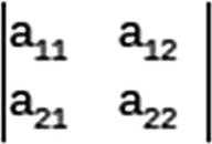
Vectors and Matrices
If we want to calculate this dot product, then a loop performing multiply and accumulate instructions will be quite efficient.
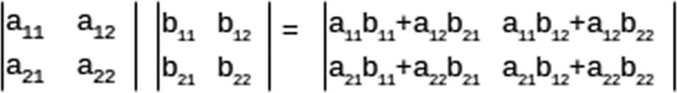

In 3D graphics, if we represent a point as a 4D vector [x, y, z, 1], then the affine transformations of scale, rotate, shear, and reflection can be represented as 4x4 matrices. Any number of these transformations can be combined into a single matrix. Thus, to transform an object into a scene requires a matrix multiplication applied to each of the object’s vertex points. The faster we can do this, the faster we can render a frame in a video game.
In neural networks, the calculation for each layer of neurons is calculated by a matrix multiplication followed by the application of a nonlinear function. The bulk of the work is the matrix multiplication. Most neural networks have many layers of neurons, each requiring a matrix multiplication. The matrix size corresponds to the number of variables and the number of neurons; consequently, the matrices’ dimensions are often in the thousands. How quickly we perform object recognition or speech translation depends on how fast we can multiply matrices, which depends on how fast we can do multiply with accumulate.
These important applications are why the ARM processor dedicates so much silicon to multiply and accumulate. We’ll keep returning to how to speed up this process as we explore the ARM CPU’s floating-point unit (FPU) and Neon coprocessors in the following chapters.
Accumulate Instructions
MADD Xd, Xn, Xm, Xa
MSUB Xd, Xn, Xm, Xa
SMADDL Xd, Wn, Wm, Xa
UMADDL Xd, Wn, Wm, Xa
SMSUBL Xd, Wn, Wm, Xa
UMSUBL Xd, Wn, Wm, Xa
The multiplication with accumulate instructions map closely to the multiply instructions that we’ve already discussed. In fact, most of the multiply instructions are aliases of these instructions using the zero register for Xa.
Xd can be the same as Xa, for calculating a running sum.
In the second case, we see that if Xa is the zero register, then we get all the multiply negative operations in the last section.
For the versions that multiple two 32-bit registers to get a 64-bit results, the sum needs to be a 64-bit X register.
Example 1
We’ve talked about how multiply and accumulate is ideal for multiplying matrices, so for an example, let’s multiply two 3x3 matrices.
Pseudo-code for our matrix multiplication program
The row and column loops go through each cell of the output matrix and calculate the correct dot product for that cell in the innermost loop.
3x3 matrix multiplication in Assembly
Accessing Matrix Elements
We store the three matrices in memory, in row order. They are arranged in the .word directives so that you can see the matrix structure. In the pseudo-code, we refer to the matrix elements using two-dimensional arrays. There are no instructions or operand formats to specify two-dimensional array access, so we must do it ourselves. To Assembly each array is just a nine-word sequence of memory. Now that we know how to multiply, we can do something like
A[i, j] = A[i∗N + j]
where N is the dimension of the array. We don’t do this though; in Assembly it pays to notice that we access the array elements in order and can go from one element in a row to the next by adding the size of an element—the size of a word, or 4 bytes. We can go from an element in a column to the next one by adding the size of a row. Therefore, we use the constant N ∗ WDSIZE so often in the code. This way we go through the array incrementally and never have to multiply array indexes. Generally, multiplication and division are expensive operations, and we should try to avoid them as much as possible.
which stores our computed dot product into C and then increments the pointer into C by 4 bytes. We see it again when we print the C matrix at the end.
Multiply with Accumulate
This instruction accumulates a 64-bit sum, though we only take the lower 32 bits when we store it into the result matrix C. We don’t check for overflow, but as long as the numbers in A and B are small, we won’t have a problem.
Register Usage
We use quite a few registers, so we’re lucky we can keep track of all our loop indexes and pointers in registers, without having to move them in and out of memory. If we had to do this, we would have allocated space on the stack to hold any needed variables.
Notice that we use registers X19 and X20 in the loop that does the printing. That is because the printf function will change any of registers X0–X18 on us. We mostly use registers X0–X18 otherwise since we don’t need to preserve these for our caller. However, we do need to preserve X19 and X20, so we push and pop these to and from the stack along with LR.
Summary
We introduced the various forms of the multiply and division instructions supported in the ARM 64-bit instruction set.
We then explained the concept of multiply and accumulate and why these instructions are so important to modern applications in graphics and machine learning. We reviewed the many variations of these instructions and then presented an example matrix multiplication program to show them in action.
In Chapter 12, “Floating-Point Operations,” we will look at more math, but this time in scientific notation allowing fractions and exponents, going beyond integers for the first time.
Exercises
- 1.
To multiply two 64-bit numbers resulting in a 128-bit product, we used the MUL instruction to obtain the lower 64 bits of the product for both the signed and unsigned integer cases. To prove that this works, let’s work a small example multiplying two 4-bit numbers to get an 8-bit product. Multiply 0xf by 2. In this signed case, 0xf is -1 and the product is -2; in the unsigned case, 0xf is 15 and the product is 30. Manually perform the calculation to ensure the correct result is obtained in both cases.
- 2.
Write a signed 64-bit integer division routine that checks if the denominator is zero before performing the division. Print an error if zero is encountered.
- 3.
Write a routine to compute a dot product of dimension six. Put the numbers to calculate in the .data section and print the result.
- 4.
Change your program in Exercise 3 to use multiply and subtract from accumulator, instead of adding.
- 5.
Change the matrices calculated in the example and check that the result is correct.