

Cost Control
15.0 INTRODUCTION
PMBOK® Guide, 4th Edition
7.3 Cost Control
Cost control is equally important to all companies, regardless of size. Small companies generally have tighter monetary controls because the failure of even one project can put the company at risk, but they have less sophisticated control techniques. Large companies may have the luxury to spread project losses over several projects, whereas the small company may have few projects.
Many people have a poor understanding of cost control. Cost control is not only “monitoring” costs and recording data, but also analyzing the data in order to take corrective action before it is too late. Cost control should be performed by all personnel who incur costs, not merely the project office.
Cost control implies good cost management, which must include:
- Cost estimating
- Cost accounting
- Project cash flow
- Company cash flow
- Direct labor costing
- Overhead rate costing
- Other tactics, such as incentives, penalties, and profit-sharing
Cost control is actually a subsystem of the management cost and control system (MCCS) rather than a complete system per se. This is shown in Figure 15-1, where the MCCS is represented as a two-cycle process: a planning cycle and an operating cycle. The operating cycle is what is commonly referred to as the cost control system. Failure of a cost control system to accurately describe the true status of a project does not necessarily imply that the cost control system is at fault. Any cost control system is only as good as the original plan against which performance will be measured. Therefore, the designing of a planning system must take into account the cost control system. For this reason, it is common for the planning cycle to be referred to as planning and control, whereas the operating cycle is referred to as cost and control.
The planning and control system must help management project the status toward objective completion. Its purpose is to establish policies, procedures, and techniques that can be used in the day-to-day management and control of projects and programs. It must, therefore, provide information that:
- Gives a picture of true work progress
- Will relate cost and schedule performance
- Identifies potential problems with respect to their sources.
- Provides information to project managers with a practical level of summarization
- Demonstrates that the milestones are valid, timely, and auditable
The planning and control system, in addition to being a tool by which objectives can be defined (i.e., hierarchy of objectives and organization accountability), exists as a tool to develop planning, measure progress, and control change. As a tool for planning, the system must be able to:
- Plan and schedule work
- Identify those indicators that will be used for measurement
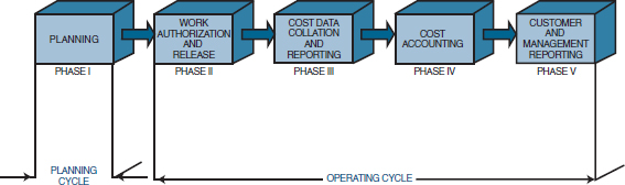
FIGURE 15-1. Phases of a management cost and control system.
The project budget that results from the planning cycle of the MCCS must be reasonable, attainable, and based on contractually negotiated costs and the statement of work. The basis for the budget is either historical cost, best estimates, or industrial engineering standards. The budget must identify planned manpower requirements, contract-allocated funds, and management reserve.
Establishing budgets requires that the planner fully understand the meaning of standards. There are two categories of standards. Performance results standards are quantitative measurements and include such items as quality of work, quantity of work, cost of work, and time-to-complete. Process standards are qualitative, including personnel, functional, and physical factors relationships. Standards are advantageous in that they provide a means for unity, a basis for effective control, and an incentive for others. The disadvantage of standards is that performance is often frozen, and employees are quite often unable to adjust to the differences.
As a tool for measuring progress and controlling change, the systems must be able to:
- Measure resources consumed
- Measure status and accomplishments
- Compare measurements to projections and standards
- Provide the basis for diagnosis and replanning
In using the MCCS, the following guidelines usually apply:
- The level of detail is specified by the project manager with approval by top management.
- Centralized authority and control over each project are the responsibility of the project management division.
- For large projects, the project manager may be supported by a project team for utilization of the MCCS.
Almost all project planning and control systems have identifiable design requirements. These include:
- A common framework from which to integrate time, cost, and technical performance
- Ability to track progress of significant parameters
- Quick response
- Capability for end-value prediction
- Accurate and appropriate data for decision-making by each level of management
- Full exception reporting with problem analysis capability
- Immediate quantitative evaluation of alternative solutions
MCCS planning activities include:
- Contract receipt (if applicable)
- Work authorization for project planning
- Work breakdown structure
- Subdivided work description
- Schedules
- Planning charts
- Budgets
MCCS planning charts are worksheets used to create the budget. These charts include planned labor in hours and material dollars.
MCCS planning is accomplished in one of these ways:
- One level below the lowest level of the WBS
- At the lowest management level
- By cost element or cost account
Even with a fully developed planning and control system, there are numerous benefits and costs. The appropriate system must consider a cost-benefit analysis, and include such items as:
- Project benefits
- Planning and control techniques facilitate:
- —Derivation of output specifications (project objectives)
- —Delineation of required activities (work)
- —Coordination and communication between organizational units
- —Determination of type, amount, and timing of necessary resources
- —Recognition of high-risk elements and assessment of uncertainties
- —Suggestions of alternative courses of action
- —Realization of effect of resource level changes on schedule and output performance
- —Measurement and reporting of genuine progress
- —Identification of potential problems
- —Basis for problem-solving, decision-making, and corrective action
- —Assurance of coupling between planning and control
- Planning and control techniques facilitate:
- Project cost
- Planning and control techniques require:
- —New forms (new systems) of information from additional sources and incremental processing (managerial time, computer expense, etc.)
- —Additional personnel or smaller span of control to free managerial time for planning and control tasks (increased overhead)
- —Training in use of techniques (time and materials)
- Planning and control techniques require:
A well-disciplined MCCS will produce the following results:
- Policies and procedures that will minimize the ability to distort reporting
- Strong management emphasis on meeting commitments
- Weekly team meetings with a formalized agenda, action items, and minutes
- Top-management periodic review of the technical and financial status
- Simplified internal audit for checking compliance with procedures
For MCCS to be effective, both the scheduling and budgeting systems must be disciplined and formal in order to prevent inadvertent or arbitrary budget or schedule changes. This does not mean that the baseline budget and schedule, once established, is static or inflexible. Rather, it means that changes must be controlled and result only from deliberate management actions.
Disciplined use of MCCS is designed to put pressure on the project manager to perform exceptionally good project planning so that changes will be minimized. As an example, government subcontractors may not:
- Make retroactive changes to budgets or costs for work that has been completed
- Rebudget work-in-progress activities
- Transfer work or budget independently of each other
- Reopen closed work packages
In some industries, the MCCS must be used on all contracts of $2 million or more, including firm-fixed-price efforts. The fundamental test of whether to use the MCCS is to determine whether the contracts have established end-item deliverables, either hardware or computer software, that must be accomplished through measurable efforts.
Two programs are used by the government and industry in conjunction with the MCCS as an attempt to improve effectiveness in cost control. The zero-base budgeting program provides better estimating techniques for the verification portion of control. The design-to-cost program assists the decision-making part of the control process by identifying a decision-making framework from which replanning can take place.
15.1 UNDERSTANDING CONTROL
PMBOK® Guide, 4th Edition
3.2 Monitoring and Control Process Group
Effective management of a program during the operating cycle requires that a well-organized cost and control system be designed, developed, and implemented so that immediate feedback can be obtained, whereby the up-to-date usage or resources can be compared to target objectives established during the planning cycle. The requirements for an effective control system (for both cost and schedule/performance) should include1:
- Thorough planning of the work to be performed to complete the project
- Good estimating of time, labor, and costs
- Clear communication of the scope of required tasks
- A disciplined budget and authorization of expenditures
- Timely accounting of physical progress and cost expenditures
- Periodic reestimation of time and cost to complete remaining work
- Frequent, periodic comparison of actual progress and expenditures to schedules and budgets, both at the time of comparison and at project completion
Management must compare the time, cost, and performance of the program to the budgeted time, cost, and performance, not independently but in an integrated manner. Being within one's budget at the proper time serves no useful purpose if performance is only 75 percent. Likewise, having a production line turn out exactly 200 items, as planned, loses its significance if a 50 percent cost overrun is incurred. All three resource parameters (time, cost, and performance) must be analyzed as a group, or else we might “win the battle but lose the war.” The use of the expression “management cost and control system” is vague in that the implication is that only costs are controlled. This is not true—an effective control system monitors schedule and performance as well as costs by setting budgets, measuring expenditures against budgets and identifying variances, assuring that the expenditures are proper, and taking corrective action when required.
Previously we defined the work breakdown structure as the element that acts as the source from which all costs and controls must emanate. The WBS is the total project broken down into successively lower levels until the desired control levels are established. The work breakdown structure therefore serves as the tool from which performance can be subdivided into objectives and subobjectives. As work progresses, the WBS provides the framework on which costs, time, and schedule/performance can be compared against the budget for each level of the WBS.
The first purpose of control therefore becomes a verification process accomplished by the comparison of actual performance to date with the predetermined plans and standards set forth in the planning phase. The comparison serves to verify that:
- The objectives have been successfully translated into performance standards.
- The performance standards are, in fact, a reliable representation of program activities and events.
- Meaningful budgets have been established such that actual versus planned comparisons can be made.
In other words, the comparison verifies that the correct standards were selected, and that they are properly used.
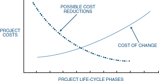
FIGURE 15-2. Cost reduction analysis.
The second purpose of control is decision-making. Three useful reports are required by management in order to make effective and timely decisions:
- The project plan, schedule, and budget prepared during the planning phase
- A detailed comparison between resources expended to date and those predetermined. This includes an estimate of the work remaining and the impact on activity completion.
- A projection of resources to be expended through program completion
These reports, supplied to the managers and the doers, provide three useful results:
- Feedback to management, the planners, and the doers
- Identification of any major deviations from the current program plan, schedule, or budget
- The opportunity to initiate contingency planning early enough that cost, performance, and time requirements can undergo corrected action without loss of resources
These reports provide management with the opportunity to minimize downstream changes by making proper corrections here and now. As shown in Figures 15-2 and 15-3, cost reductions are more available in the early project phases, but are reduced as we go further into the project life-cycle phases. Figure 15-3 identifies the people that most likely have the greatest influence on possibly initiating changes to a project. Downstream the cost of changes could easily exceed the original cost of the project. This is an example of the “iceberg” syndrome, where problems become evident too late in the project to be solved easily, resulting in a very high cost to correct them.
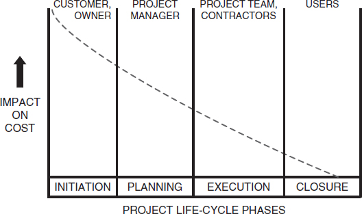
FIGURE 15-3. People with the ability to influence cost.
15.2 THE OPERATING CYCLE
The management cost and control system (MCCS) takes on paramount importance during the operating cycle of the project. The operating cycle is composed of four phases:
- Work authorization and release (phase II)
- Cost data collection and reporting (phase III)
- Cost analysis (phase IV)
- Reporting: customer and management (phase V)
These four phases, when combined with the planning cycle (phase I), constitute a closed system network that forms the basis for the management cost and control system.
Phase II is considered as work release. After planning is completed and a contract is received, work is authorized via a work description document. The work description, or project work authorization form, is a contract that contains the narrative description, organization, and time frame for each WBS level. This multipurpose form is used to release the contract, authorize planning, record detail description of the work outlined in the work breakdown structure, and release work to the functional departments.
Contract services may require a work description form to release the contract. The contractual work description form sets forth general contractual requirements and authorizes program management to proceed.
Program management may then issue a subdivided work description form to the functional units so that work can begin. The subdivided work description may also be issued through the combined efforts of the project team, and may be revised or amended when either the scope or the time frame changes. The subdivided work description generally is not used for efforts longer than ninety days and must be “tracked” as if a project in itself. This subdivided work description form sets forth contractual requirements and planning guidelines for the applicable performing organizations. The subdivided work description package established during the proposal and updated after negotiations by the program team is incrementally released by program management to the work control centers in manufacturing, engineering, publications, and program management as the authority for release of work orders to the performing organizations. The subdivided work description specifies how contractual requirements are to be accomplished, the functional organizations involved, and their specific responsibilities, and authorizes the expenditure of resources within a particular time frame.
The work control center assigns a work order number to the subdivided work description form, if no additional instructions are required, and releases the document to the performing organizations. If additional instructions are required, the work control center can prepare a more detailed work-release document (shop traveler, tool order, work order release), assign the applicable work order number, and release it to the performing organization.
A work order number is required for all in-house direct and indirect charging. The work order number also serves as a cross-reference number for automatic assignment of the indentured work breakdown structure number to labor and material data records in the computer.
Small companies can avoid this additional paperwork cost by going directly from an awarded contract to a single work order, which may be the only work order needed for the entire contract.
15.3 COST ACCOUNT CODES
PMBOK® Guide, 4th Edition
7.2.2.1 Cost Aggregation
Since project managers control resources through the line managers rather than directly, project managers end up controlling direct labor costs by opening and closing work orders. Work orders define the charge numbers for each cost account. By definition, a cost account is an identified level at a natural intersection point of the work breakdown structure and the organizational breakdown structure (OBS) at which functional responsibility for the work is assigned, and actual direct labor, material, and other direct costs are compared with actual work performed for management control purposes.
Cost accounts are the focal point of the MCCS and may comprise several work packages, as shown in Figure 15-4. Work packages are detailed short-span job or material items identified for the accomplishment of required work. To illustrate this, consider the cost account code breakdown shown in Figure 15-5 and the work authorization form shown in Figure 15-6. The work authorization form specifically identifies the cost centers that are “open” for this charge number, the man-hours available for each cost center, and the operational time period for the charge number. Because the exact dates of operation are completely defined, the charge number can be assigned perhaps as much as a year in advance of the work-begin date. This can be shown pictorially, as in Figure 15-7.
If the man-hours are assigned to Cost Center 2400, then any 24xx cost center can use this charge number. If the work authorization form specifies Cost Center 2610, then any 261x cost center can use the charge number. However, if Cost Center 2623 is specified, then no lower cost accounts exist, and this is the only cost center that can use this work order charge number. In other words, if a charge number is opened up at the department level, then the department manager has the right to subdivide the assigned man-hours among the various sections and subsections. Company policy usually identifies the permissible cost center levels that can be assigned in the work authorization form. These permissible levels are related to the work breakdown structure level. For example, Cost Center 5000 (i.e., divisional) can be assigned at the project level of the work breakdown structure, but only department, sectional, or subsectional cost accounts can be assigned at the task level of the work breakdown structure.
If a cost center needs additional time or additional man-hours, then a cost account change notice form must be initiated, usually by the requesting cost center, and approved by the project office. Figure 15-8 shows a typical cost account change notice form.
Large companies have computerized cost control and reporting systems. Small companies have manual or partially computerized systems. The major difficulty in using the cost account code breakdown and the work authorization form (Figures 15-5 and 15-6) is related to whether the employees fill out time cards, and frequency with which the time cards are filled out. Project-driven organizations fill out time cards at least once a week, and the cards are inputted to a computerized system. Non-project-driven organizations fill out time cards on a monthly basis, with computerization depending on the size of the company.
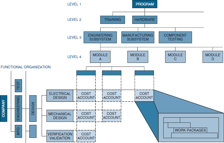
FIGURE 15-4. The cost account intersection.
PMBOK® Guide, 4th Edition
7.2.2.1 Cost Aggregation
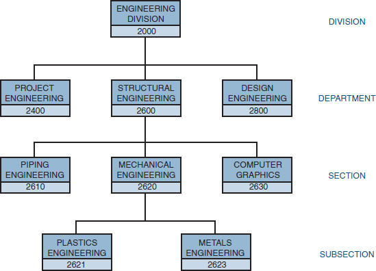
FIGURE 15-5. Cost account code breakdown.
PMBOK® Guide, 4th Edition
4.4 Monitor and Control Project Work
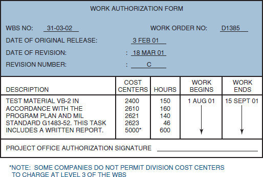
FIGURE 15-6. Work authorization form.
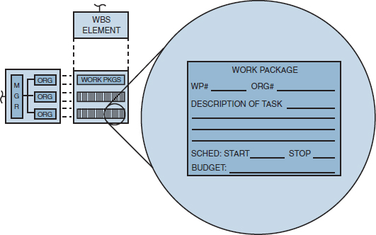
FIGURE 15-7. Planning and budgeting describe, plan, and schedule the work.
Cost data collection and reporting constitute the second phase of the operating cycle of the MCCS. Actual cost (ACWP) and the budgeted cost for work performed (BCWP) for each contract or in-house project are accumulated in detailed cost accounts by cost center and cost element, and reported in accordance with the flow charts shown in Figure 15-9. These detailed elements, for both actual costs incurred and the budgeted cost for work performed, are usually printed out monthly for all levels of the work breakdown structure. In addition, weekly supplemental direct labor reports can be printed showing the actual labor charge incurred, and can be compared to the predicted efforts.
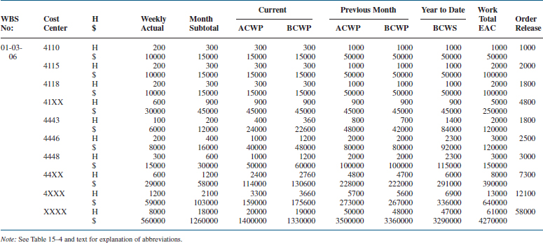
Table 15-1 shows a typical weekly labor report. The first column identifies the WBS number.2 If more than one work order were assigned to this WBS element, then the work order number would appear under the WBS number. This procedure would be repeated for all work orders under the same WBS number. The second column contains the cost centers charging to this WBS element (and possibly work order numbers). Cost Center 41xx represents department 41 and is a rollup of Cost Centers 4110, 4115, and 4118. Cost Center 4xxx represents the entire division and is a rollup of all 4000-level departments. Cost Center xxxx represents the total for all divisions charging to this WBS element. The weekly labor reports must list all cost centers authorized to charge to this WBS element, whether or not they have incurred any costs over the last reporting period.
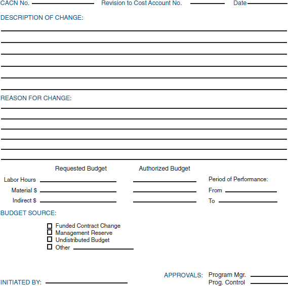
FIGURE 15-8. Cost account change notice (CACN).
Most weekly labor reports provide current month subtotals and previous month totals. Although these also appear on the detailed monthly report, they are included in the weekly report for a quick-and-dirty comparison. Year-to-date totals are usually not on the weekly report unless the users request them for an immediate comparison to the estimate at completion (EAC) and the work order release.
Weekly labor output is a vital tool for members of the program office in that these reports can indicate trends in cost and performance in sufficient time for contingency plans to be established and implemented. If these reports are not available, then cost and labor overruns would not be apparent until the following month when the detailed monthly labor, cost, and materials output was obtained.
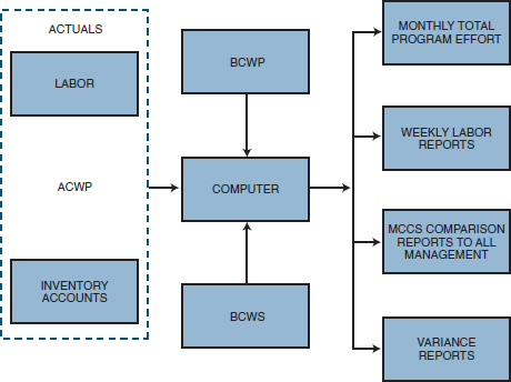
FIGURE 15-9. Cost data collection and reporting flowchart.
In Table 15-1, Cost Center 4110 has spent its entire budget. The work appears to be completed on schedule. The responsible program office team may wish to eliminate this cost center's authority to continue charging to this WBS element by issuing a new subdivided work description or work order canceling this department's efforts. Cost Center 4115 appears to be only halfway through. If time is becoming short, then Cost Center 4115 must add resources in order to meet requirements. Cost Center 4443 appears to be heading for an overrun. This could also indicate a management reserve. In this case the responsible program team member feels that the work can be accomplished in fewer hours.
Work order releases are used to authorize certain cost centers to begin charging their time to a specific cost reporting element. Work orders specify hours, not dollars. The hours indicate the “targets” that the program office would like to have the department shoot for. If the program office wished to be more specific and “compel” the departments to live within these hours, then the budgeted cost for work scheduled (BCWS) should be changed to reflect the reduced hours.
Four categories of cost data are normally accumulated:
- Labor
- Material
- Other direct charges
- Overhead
Project managers can maintain reasonable control over labor, material, and other direct charges. Overhead costs, on the other hand, are calculated yearly or monthly and applied retroactively to all applicable programs. Management reserves are often used to counterbalance the effects of adverse changes in overhead rates.
TABLE 15-1. WEEKLY LABOR REPORT
15.4 BUDGETS
The project budget, which is the final result of the planning cycle of the MCCS, must be reasonable, attainable, and based on contractually negotiated costs and the statement of work. The basis for the budget is either historical cost, best estimates, or industrial engineering standards. The budget must identify planned manpower requirements, contract allocated funds, and management reserve.
All budgets must be traceable through the budget “log,” which includes:
- Distributed budget
- Management reserve
- Undistributed budget
- Contract changes
The distributed or normal performance budget is the time-phased budget that is released through cost accounts and work packages. Management reserve is generally the dollar amount established for categories of unforeseen problems and contingencies resulting in special out-of-scope work to the performers. Sometimes, people interpret the management reserve as their own little kitty of funds for a special purpose. Below are several interpretations on how the control of the management reserve should be used.
- The management reserve is actually excess profits and should not be used at all. It should be booked as additional profits as soon as possible. (Accounting)
- The management reserve should be spent on any activities that add features or additional functionality to the product. Our customers will like that. It will also build up good customer relations for future work. (Marketing)
- The management reserve should be used for those activities that add value to our company, especially our image in the community. (Senior management)
- The management reserve should be use as part of risk management in developing mitigation strategies for risks that occur during the execution of the project. Scope changes not originally agreed to should be billed separately to the customer. (Project manager)
- The management reserve should be used for the additional hours necessary to show that our technical community can exceed specifications rather than merely meeting them. This is our strength. The management reserve should also be used as “seed money” for exploring ideas discovered while working on this project. (Engineering and R&D)
Some people confuse the management reserve with the definition of a “reserve” or “contingency” fund. In the author's opinion, the management reserve is controlled by the project manager of the performing organization and used for escalations in salaries, raw material prices, and overhead rates. The management reserve may also be used for unforeseen problems that may occur. The management reserve should not be used to cover up bad planning estimates or budget overruns.
Also, the management reserve should not be used for scope changes. Scope changes should be paid for out of the customer's reserve or contingency fund. In other words, the management reserve generally applies to the performing organization, whereas the contingency reserve is controlled by the customer for the scope changes that may be requested by the performing organization. There is an exception. If the performing organization is requesting a small scope change, the cost of convening the change control board, paying airfares, meals, and lodgings may be prohibited. In this case, the management reserve may be used and considered as a goodwill activity for the performing organization.
The management reserve should be established based upon the project's risks. Some project may require no management reserve at all, whereas others may necessitate a reserve of 15 percent.
There is always the question of who should get to keep any unused management reserve at the end of the project. If the project is under a firm-fixed price contract, then the management reserve becomes extra profit for the performing organization. If the contract is a cost reimbursable type, all or part of the unused management reserve may have to be returned to the customer.
Although the management reserve may appear as a line item in the work breakdown structure, it is neither part of the distributed budget nor part of the cost baseline. Budgets are established on the assumption that they will be spent, whereas management reserve is money that you try not to spend. It would be inappropriate to consider the management reserve as an undistributed budget.
In addition to the “normal” performance budget and the management reserve budget, there are two other budgets:
- Undistributed budget, which is that budget associated with contract changes where time constraints prevent the necessary planning to incorporate the change into the performance budget. (This effort may be time-constrained.)
- Unallocated budget, which represents a logical grouping of contract tasks that have not yet been identified and/or authorized.
15.5 THE EARNED VALUE MEASUREMENT SYSTEM (EVMS)
In the early years of project management, it became evident that project managers were having difficulty determining project status. Some people believed that status could be determined only by a mystical approach, as shown in Figure 15-10.
The critical question was whether project managers were managing costs or just monitoring costs. The government wanted costs to be managed rather than just monitored, accounted for, or reported. This need resulted in the creation of the EVMS.
The basis for the EVMS, which some consider to be a component of the MCCS, is the determination of earned value. Earned value is a management technique that relates resource planning to schedules and technical performance requirements. Earned value management (EVM) is a systematic process that uses earned value as the primary tool for integrating cost, schedule, technical performance management, and risk management.

FIGURE 15-10. Determining the status.
Without using the EVMS, determining status can be difficult. Consider the following:
- The project
- A total budget of $1.2 million
- A 12-month effort
- Produce 10 deliverables
- Reported status
- Time elapsed: 6 months
- Money spent to date: $700,000
- Deliverables produced: 4 complete, 2 partial
What is the real status of the project? How far along is the project: 40, 50, 60 percent, etc.? Another problem was how to accurately relate cost to performance. If you spent 20 percent of the budget, does that imply that you are 20 percent complete? If you are 30 percent complete, then have you spent 30 percent of the budget?
The EVMS provides the following benefits:
- Accurate display of project status
- Early and accurate identification of trends
- Early and accurate identification of problems
- Basis for course corrections
The EVMS can answer the following questions:
- What is the true status of the project?
- What are the problems?
- What can be done to fix the problems?
- What is the impact of each problem?
- What are the present and future risks?
The EVMS emphasizes prevention over cures by identifying and resolving problems early. The EVMS is an early warning system allowing for early identification of trends and variances from the plan. The EVMS provides an early warning system, thus allowing the project manager sufficient time to make course corrections in small increments. It is usually easier to correct small variances as opposed to large variances. Therefore, the EVMS should be used continuously throughout the project in order to detect the variances while they are small and possibly easy to correct. Large variances are more difficult to correct and run the risk that the cost to correct the large variance may displease management to the point where the project may be canceled.
15.6 VARIANCE AND EARNED VALUE
A variance is defined as any schedule, technical performance, or cost deviation from a specific plan. Variances must be tracked and reported. They should be mitigated through corrective actions and not eliminated through a baseline change unless there is a good reason. Variances are used by all levels of management to verify the budgeting system and the scheduling system. The budgeting and scheduling system variance must be compared because:
- The cost variance compares deviations only from the budget and does not provide a measure of comparison between work scheduled and work accomplished.
- The scheduling variance provides a comparison between planned and actual performance but does not include costs.
There are two primary methods of measurement:
- Measurable efforts: Discrete increments of work with a definable schedule for accomplishment, whose completion produces tangible results.
- Level of effort: Work that does not lend itself to subdivision into discrete scheduled increments of work, such as project support and project control.
Variances are used on both types of measurement.
In order to calculate variances, we must define the three basic variances for budgeting and actual costs for work scheduled and performed. Archibald defines these variables3:
- Budgeted cost for work scheduled (BCWS) is the budgeted amount of cost for work scheduled to be accomplished plus the amount or level of effort or apportioned effort scheduled to be accomplished in a given time period.
PMBOK® Guide, 4th Edition
7.3.2 Cost Control Tools and Techniques
7.3.2.4 Performance Measurement Analysis
- Budget cost for work performed (BCWP) is the budgeted amount of cost for completed work, plus budgeted for level of effort or apportioned effort activity completed within a given time period. This is sometimes referred to as “earned value.”
- Actual cost for work performed (ACWP) is the amount reported as actually expended in completing the work accomplished within a given time period.
Note: The Project Management Institute has changed the nomenclature in their new version of the PMBOK® Guide whereby BCWS is now PV, BCWP is now EV, and ACWP is now AC. However, the majority of heavy users of these acronyms, specifically government contractors, still use the old acronyms. Until the PMI acronyms are accepted across all industries, we will continue to focus on the most commonly used acronyms.
BCWS represents the time-phased budget plan against which performance is measured. For the total contract, BCWS is normally the negotiated contract plus the estimated cost of authorized but unpriced work (less any management reserve). It is time-phased by the assignment of budgets to scheduled increments of work. For any given time period, BCWS is determined at the cost account level by totaling budgets for all work packages, plus the budget for the portion of in-process work (open work packages), plus the budget for level of effort and apportioned effort.
A contractor must utilize anticipated learning when developing the time-phased BCWS. Any recognized method used to apply learning is usually acceptable as long as the BCWS is established to represent as closely as possible the expected actual cost (ACWP) that will be charged to the cost account/work package.
These costs can then be applied to any level of the work breakdown structure (i.e., program, project, task, subtask, work package) for work that is completed, in-program, or anticipated. Using these definitions, the following variance definitions are obtained:
- Cost variance (CV) calculation:
CV = BCWP − ACWP
A negative variance indicates a cost-overrun condition.
- Schedule variance (SV) calculation:
SV = BCWP − BCWS
A negative variance indicates a behind-schedule condition.
In the analysis of both cost and schedule, costs are used as the lowest common denominator. In other words, the schedule variance is given as a function of cost. To alleviate this problem, the variances are usually converted to percentages:
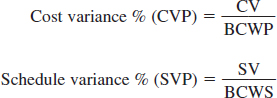
The schedule variance may be represented by hours, days, weeks, or even dollars.
As an example, consider a project that is scheduled to spend $100K for each of the first four weeks of the project. The actual expenditures at the end of week four are $325K. Therefore, BCWS = $400K and ACWP = $325K. From these two parameters alone, there are several possible explanations as to project status. However, if BCWP is now known, say $300K, then the project is behind schedule and overrunning costs.
It is important to understand the physical meaning of CV and SV. Consider the following example:
- BCWS = $1000
- BCWP = $800
- ACWP = $700
In this example, the units are dollars. The units could have just as easily been hours, days, or weeks. In this example, CV = $800 − $700 = +$100. Because CV is a positive value, it indicates that physical progress was accomplished at a lower cost than the forecasted cost. This is a favorable situation. Had CV been negative, it would have indicated that physical progress was accomplished at a greater cost than what was forecasted. If CV = 0, then the physical accomplishment was as budgeted.
Although CV is measured in hours or dollars, it is actually a measurement of the efficiency with which physical progress was accomplished compared with the plan. To correct a negative cost variance, emphasis should be placed upon the productivity rate (i.e., burn rate) at which work is being performed.
Returning to the above example, SV = $800 − $1000 = −$200. In this example, the schedule variance is a negative value, indicating that physical progress is being accomplished at a slower rate than planned. This is an unfavorable condition. If the schedule variance were positive, this would indicate physical progress being accomplished at a faster rate than planned. If SV = 0, physical progress is being accomplished as planned.
The schedule variance, SV, measures the timeliness of the physical progress compared to the plan whereas the cost variance, CV, measures the efficiency. To correct a negative schedule variance, emphasis should be placed upon improving the speed by which work is being performed.
The cost variance relates to the real cost. However, the problem with SV is how it relates to the real schedule. The schedule variance is determined from cost account or work package financial numbers and does not necessarily relate to the real schedule. The schedule variance does not distinguish between critical path and non-critical path work packages. The schedule variance by itself does not measure time. A negative schedule variance indicates a behind-schedule condition but does not mean that the critical path has slipped. On the contrary, the real schedule (i.e., precedence networks or the arrow diagramming networks) could indicate that the project will be ahead of schedule. A detailed analysis of the real schedule is still required irrespective of the value for the schedule variance.
Variances are almost always identified as critical items and are reported to all organizational levels. Critical variances are established for each level of the organization in accordance with management policies.
Not all companies have a uniform methodology for variance thresholds. Permitted variances may be dependent on such factors as:
- Life-cycle phase
- Length of life-cycle phase
- Length of project
- Type of estimate
- Accuracy of estimate
Variance controls may be different from program to program. Table 15-2 identifies sample variance criteria for program X.
For many programs and projects, variances are permitted to change over the duration of the program. For strict manufacturing programs (product management), variances may be fixed over the program time span using criteria as in Table 15-2. For programs that include research and development, larger deviations may be permitted during the earlier phases than during the later phases. Figure 15-11 shows time-phased cost variances for a program requiring research and development, qualification, and production phases. Since the risk should decrease as time goes on, the variance boundaries are reduced. Figure 15-12 shows that the variance envelope in such a case may be dependent on the type of estimate.
By using both cost and schedule variance, we can develop an integrated cost/schedule reporting system that provides the basis for variance analysis by measuring cost performance in relation to work accomplished. This system ensures that both cost budgeting and performance scheduling are constructed on the same database.
In addition to calculating the cost and schedule variances in terms of dollars or percentages, we also want to know how efficiently the work has been accomplished. The formulas used to calculate the performance efficiency as a percentage of EV are:
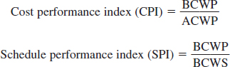
TABLE 15-2. VARIANCE CONTROL FOR PROGRAM X
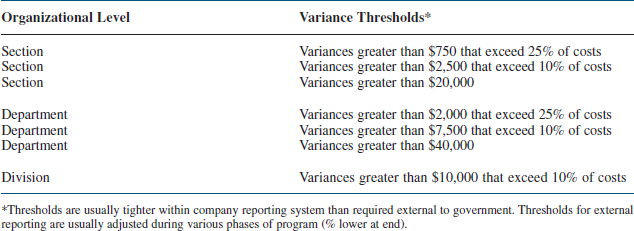
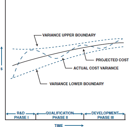
FIGURE 15-11. Project variance projection.
If CPI = 1.0, we have perfect cost performance. If CPI < 1.0, physical progress is being accomplished at a greater cost than forecasted. This is unfavorable. If CPI > 1.0, physical progress is being accomplished at less than the forecasted cost, which is favorable. Similar to CV, CPI measures the efficiency by which the physical progress was accomplished compared to the plan or baseline. For an unfavorable value of CPI, emphasis should be placed upon improving the productivity by which work was being performed.
If SPI = 1.0, we have perfect schedule performance. If SPI < 1.0, physical progress was accomplished at a slower rate than what was planned. This is unfavorable. If SPI > 1.0, physical progress was accomplished at a faster rate than what was planned, which is favorable. For an unfavorable value of SPI, emphasis should be placed upon improving the timeliness of the physical progress.
SPI and CPI are expressed as ratios compared to the performance factor of 1.0 whereas CV and SV are expressed in hours or dollars. One historic reason for this is that SPI and CPI can be used to show performance for a specified time period or trends over a long time horizon without disclosing actual company sensitive numbers. This makes SPI and CPI valuable tools for customer status reporting without disclosing hard numbers.
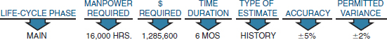
FIGURE 15-12. Methodology to variance.
The cost and schedule performance index is most often used for trend analysis as shown in Figure 15-13. Companies use either three-month, four-month, or six-month moving averages to predict trends. Trend analysis provides an early warning system and allows managers to take corrective action. Unfortunately, its use may be restricted to long-term projects because of the time needed to correct the situation.
Figure 15-14 shows an integrated cost/schedule system. The figure identifies a performance slippage to date. This might not be a bad situation if the costs are proportionately underrun. However, from the upper portion of Figure 15-14, we find that costs are overrun (in comparison to budget costs), thus adding to the severity of the situation.
Also shown in Figure 15-14 is the management reserve. This is identified as the difference between the contracted cost for projected performance to date and the budgeted cost. Management reserves are the contingency funds established by the program manager to counteract unavoidable delays that can affect the project's critical path. Management reserves cover unforeseen events within a defined project scope, but are not used for unlikely major events or changes in scope. These changes are funded separately, perhaps through management-established contingency funds. Actually, there is a difference between management reserves (which come from project budgets) and contingency funds (which come from external sources) although most people do not differentiate. It is a natural tendency for a functional manager (and some project managers) to substantially inflate estimates to protect the particular organization and provide a certain amount of cushion. Furthermore, if the inflated budget is approved, managers will undoubtedly use all of the allocated funds, including reserves. According to Parkinson4:
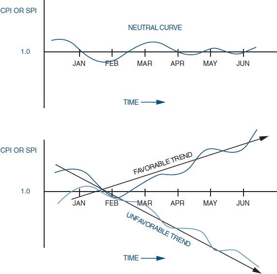
FIGURE 15-13. The performance index.
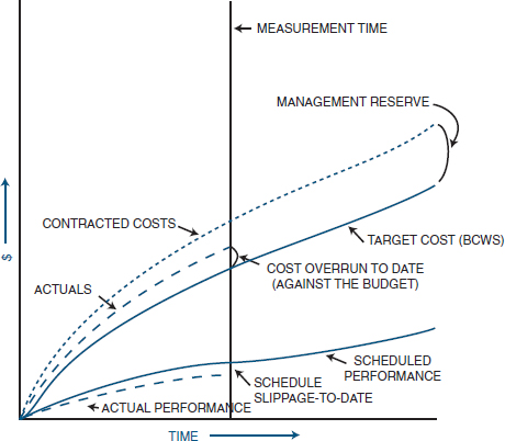
FIGURE 15-14. Integrated cost/schedule system.
- The work at hand expands to fill the time available.
- Expenditures rise to meet budget.
Managers must identify all such reserves for contingency plans, in time, cost, and performance (i.e., PERT slack time).
The line indicated as actual cost in Figure 15-14 shows a cost overrun compared to the budget. However, costs are still within the contractual requirement if we consider the management reserve. Therefore, things may not be as bad as they seem.
Government subcontractors are required to have a government-approved cost/schedule control system. The information requirements that must be demonstrated by such a system include:
- Budgeted cost for work scheduled (BCWS)
- Budgeted cost for work performed (BCWP)
- Actual cost for work performed (ACWP)
- Estimated cost at completion
- Budgeted cost at completion
- Cost and schedule variances/explanations
- Traceability
The last two items imply that standardized policies and procedures should exist for reporting and controlling variances.
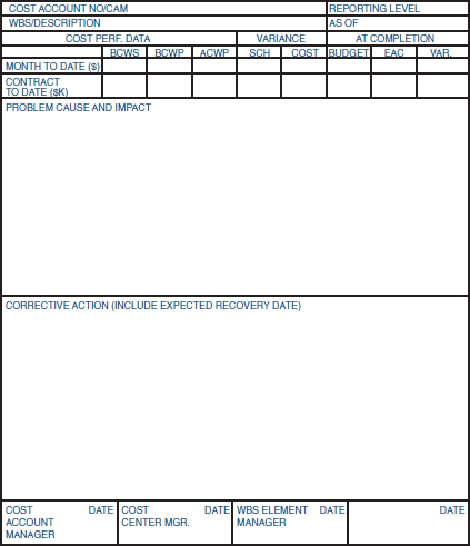
When permitted variances are exceeded, cost account variance analysis reports, as shown in Figure 15-15, are required. Required signatures may include:
- The functional employees responsible for the work
- The functional managers responsible for the work
- The cost accountant and/or the assistant project manager for cost control
- The project manager, work breakdown structure element manager, or someone with signature authority from the project office
For variance analysis, the goal of the cost account manager (whether project officer or functional employee) is to take action that will correct the problem within the original budget or justify a new estimate.
Five questions must be addressed during variance analysis:
- What is the problem causing the variance?
- What is the impact on time, cost, and performance?
- What is the impact on other efforts, if any?
- What corrective action is planned or under way?
- What are the expected results of the corrective action?
One of the key parameters used in variance analysis is the “earned value” concept, which is the same as BCWP. Earned value is a forecasting variable used to predict whether the project will finish over or under the budget. As an example, on June 1, the budget showed that 800 hours should have been expended for a given task. However, only 600 hours appeared on the labor report. Therefore, the performance is (800/600) × 100, or 133 percent, and the task is underrunning in performance. If the actual hours were 1,000, the performance would be 80 percent, and an overrun would be occurring.
The major difficulty encountered in the determination of BCWP is the evaluation of in-process work (work packages that have been started but have not been completed at the time of cutoff for the report). The use of short-span work packages or establishment of discrete value milestones within work packages will significantly reduce the work-in-process evaluation problem, and procedures used will vary depending on work package length. For example, some contractors prefer to take no BCWP credit for a short-term work package until it is completed, while others take credit for 50 percent of the work package budget when it starts and the remaining 50 percent at completion. Some contractors use formulas that approximate the time-phasing of the effort, others use earned standards, while still others prefer to make physical assessments of the work completed to determine the applicable budget earned. For longer work packages, many contractors use discrete milestones with preestablished budget or progress values to measure work performed.
The difficulty in performing variance analysis is the calculation of BCWP because one must predict the percent complete. The simplest formula for calculating BCWP is:
BCWP = (% complete) × BAC
Most people calculate “percent complete” based upon task durations. However, a more accurate representation would be to calculate “percent work complete.” However, this requires a schedule that is resource loaded. To eliminate this problem, many companies use standard dollar expenditures for the project, regardless of percent complete. For example, we could say that 10 percent of the costs are to be “booked” for each 10 percent of the time interval. Another technique, and perhaps the most common, is the 50/50 rule:
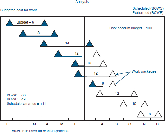
FIGURE 15-16. Analysis showing use of 50/50 rule.
Half of the budget for each element is recorded at the time that the work is scheduled to begin, and the other half at the time that the work is scheduled to be completed. For a project with a large number of elements, the amount of distortion from such a procedure is minimal. (Figures 15-16 and 15-17 illustrate this technique.)
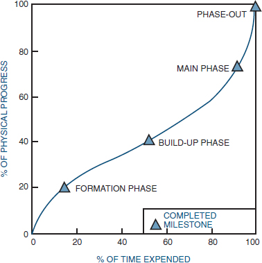
One advantage of using the 50/50 rule is that it eliminates the necessity for the continuous determination of the percent complete. However, if percent complete can be determined, then percent complete can be plotted against time expended, as shown in Figure 15-18.
There are techniques available other than the 50/50 rule5:
- 0/100: Usually limited to work packages (activities) of small duration (i.e., less than one month). No value is earned until the activity is complete.
- Milestone: This is used for long work packages with associated interim milestones, or a functional group of activities with a milestone established at identified control points. Value is earned when the milestone is completed. In these cases, a budget is assigned to the milestone rather than the work packages.
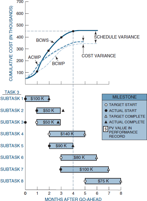
FIGURE 15-17. Project Z, task 3 cost data (contractual).
- Percent complete: Usually invoked for long-duration work packages (i.e., three months or more) where milestones cannot be identified. The value earned would be the reported percent of the budget.
- Equivalent units: Used for multiple similar-unit work packages, where earnings are on completed units, rather than labor.
- Cost formula (80/20): A variation of percent complete for long-duration work packages.
- Level of effort: This method is based on the passage of time, often used for supervision and management work packages. The value earned is based on time expended over total scheduled time. It is measured in terms of resources consumed over a given period of time and does not result in a final product.
- Apportioned effort: A rarely used technique, for special related work packages. As an example, a production work package might have an apportioned inspection work package of 20 percent. There are only a few applications of this technique. Many people will try to use this for supervision, which is not a valid application. This technique is used for effort that is not readily divisible into short-span work packages but that is in proportion to some other measured effort.
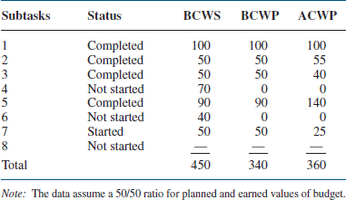
Generally speaking, the concept of earned value may not be an effective control tool if used in the lower levels of the WBS. Task levels and above are normally worth the effort for the calculation of earned value. As an example, consider Figure 15-17, which shows the contractual cost data for task 3 of project Z, and Table 15-3, which shows the cost data status at the end of the fourth month. The following is a brief summary of the cost data for each subtask in task 3 at the end of the fourth month:
- Subtask 1: All contractual funds were budgeted. Cost/performance was on time as indicated by the milestone position. Subtask is complete.
- Subtask 2: All contractual funds were budgeted. A cost overrun of $5,000 was incurred, and milestone was completed later than expected. Subtask is completed.
- Subtask 3: Subtask is completed. Costs were underrun by $10,000, probably because of early start.
TABLE 15-3. PROJECT Z, TASK 3 COST DATA STATUS AT END OF FOURTH MONTH (COST IN THOUSANDS)
- Subtask 4: Work is behind schedule. Actually, work has not yet begun.
- Subtask 5: Work is completed on schedule, but with a $50,000 cost overrun.
- Subtask 6: Work has not yet started. Effort is behind schedule.
- Subtask 7: Work has begun and appears to be 25 percent complete.
- Subtask 8: Work has not yet started.
To complete our analysis of the status of a project, we must determine the budget at completion (BAC) and the estimate at completion (EAC). Table 15-4 shows the parameters for variance analysis.
- The budget at completion is the sum of all budgets (BCWS) allocated to the project. This is often synonymous with the project baseline. This is what the total effort should cost.
- The estimate at completion identifies either the dollars or hours that represent a realistic appraisal of the work when performed. It is the sum of all direct and indirect costs to date plus the estimate of all authorized work remaining (EAC = cumulative actuals + the estimate-to-complete).
Using the above definitions, we can calculate the variance at completion (VAC):
VAC = BAC − EAC
TABLE 15-4. THE PARAMETERS FOR VARIANCE ANALYSIS
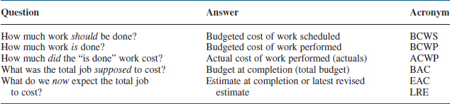
The estimate at completion (EAC) is the best estimate of the total cost at the completion of the project. The EAC is a periodic evaluation of the project status, usually on a monthly basis or until a significant change has been identified. It is usually the responsibility of the performing organization to prepare the EAC.
The calculation of a new EAC and subsequent revision does not imply that corrective action has been taken. Consider a three-month task that is 99 percent complete and was budgeted to spend $400K (BCWS). The actual costs to date (ACWP) are $395K. Using the 50/50 rule, BCWP is $200K. The estimated cost-to-complete (EAC) ratio is $395K/$200K, which implies that we are heading for a 100 percent cost overrun. Obviously, this is not the case.
Using the data in Table 15-5, we can calculate the estimate at completion (EAC) by the expression

where BAC is the value of BCWS at completion.
The discussion of what value to use for BAC is argumentative. In the above calculation, we used burdened direct labor dollars. Some people prefer to use nonburdened labor with the argument that the project manager controls only direct labor hours and dollars. Also, the calculation for EAC did not include material costs or general and administrative costs.
The above calculation of EAC implies that we are overrunning labor costs by 6.38% and that the final burdened labor cost will exceed the budgeted burdened labor cost by $34,059. For a more precise calculation of EAC we would need to include material cost (assumed at $70,000) and G&A. This would give us a final cost, excluding profit, of $751,365, which is an overrun of $37,365. The resulting profit would be $86,000 less $37,365, or $48,635. The final analysis is that work is being accomplished almost on schedule except for subtask 4 and subtask 6, but costs are being overrun.
The question that remains is, “Where is the cost overrun occurring?” To answer this question, we must analyze the cost summary sheet for project Z, task 3. Table 15-5 represents a hypothetical case for the cost elements of project Z, task 3. From Table 15-5 we see that negative (overrun) variances exist for labor dollars, overhead dollars, and material costs. Because labor overhead is measured as a percentage of direct labor dollars, the problem appears to be in the direct labor dollars.
From the contractual column in Table 15-5 the project was estimated at $27.86 per hour direct labor ($241,000/8650 hours), but actuals to date are $150,000/4652 hours, or $32.24 per hour. Therefore, higher-salaried people than anticipated are being employed. This salary increase is partially offset by the fact that there exists a positive variance of 409 direct labor hours, indicating that these higher-salaried employees are performing at a more favorable position than expected on the learning curve. Since the milestones (from Figure 15-17) appear to be on target, work is progressing as planned, except for subtask 4.
TABLE 15-5. PROJECT Z, TASK 3 COST SUMMARY FOR WORK COMPLETED OR IN PROGRESS (COST IN THOUSANDS)
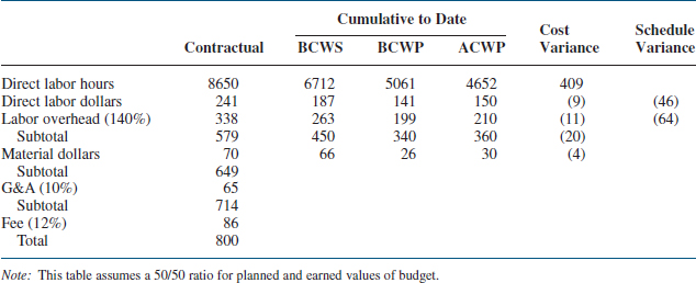
The labor overhead rate has not changed. The contractual, BCWS, and BCWP overhead rates were estimated at 140 percent. The actuals, obtained from month-end reports, indicate that the true overhead rate is as predicted.
The following conclusions can be drawn:
- Work is being performed as planned (almost on schedule, although at a more favorable position on the learning curve), except for subtask 4, which is giving us a schedule delay.
- Direct labor costs are increasing through the use of higher-salaried employees.
- Overhead rates are as anticipated.
- Direct labor hours must be reduced even further to compensate for increased costs, or profits will be drastically reduced.
This type of analysis could have been carried out to one more level by identifying exactly which departments were using the more expensive employees. This step should probably be completed anyway to see if lower-paid employees are available and can work at the required position on the learning curve. Had the labor costs been a result of increased labor hours, this step would have definitely been necessary to identify the reason for the overrun in-house. Perhaps poor estimating was the cause.
In Table 15-5, there also appears a positive variance in materials. This likewise should undergo further analysis. The cause may be the result of improperly identified hardware, material escalation costs increasing beyond what was planned, increased scrap factors, or a change in subcontractors.
It should be obvious from the above analysis that a detailed investigation into the cause of variances appears to be the best method for identifying causes. The concept of earned value, although a crude estimate, identifies trends concerning the status of specific WBS elements. Using this concept, the budgeted cost for work scheduled (BCWS) may be called planned earned value (PEV), and the budgeted cost for work performed (BCWP) may be referred to as actual earned value (AEV). Earned values are used to determine whether costs are being incurred faster or slower than planned. However, cost overruns do not necessarily mean that there will be an eventual overrun, because the work may be getting done faster than planned.
There are several formulas that can be used to calculate EAC. Using the data shown below, we can illustrate how each of three different formulas can give a different result. Assume that your project consists of these three activities only.
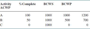
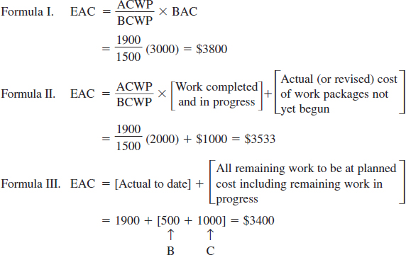
Advantages and disadvantages exist for each formula. Formula I assumes that the burn rate (i.e., ACWP/BCWP) will be the same for the remainder of the project. This is the easiest formula to use. The burn rate is updated each reporting period.
Formula II assumes that all work packages not yet opened will be completed at the planned cost. However, it is possible for planned cost to be revised based upon history from completed work packages.
Formula III assumes that all remaining work is independent of the burn rate incurred thus far. This may be unrealistic unless all remaining work can be reestimated if necessary.
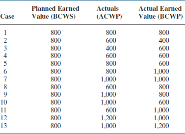
TABLE 15-6. VARIANCE ANALYSIS CASE STUDIES
Other techniques are available for determining final completion costs.6 The value of the technique selected is based upon the dollar value of the project, the risk, the quality of the cost accounting system, and the accuracy of the estimates. The estimating techniques here use only labor costs. Material costs can be added into each equation to obtain total cost.
Thirteen cases for comparing planned versus actual performance are shown in Table 15-6. Each case is described below using the relationships:
- Cost variance = actual earned value − actuals
- Schedule/performance variances = actual earned value − planned earned value
Case 1: This is the ideal planning situation where everything goes according to schedule.
Case 2: Costs are behind schedule, and the program appears to be underrunning. Work is being accomplished at less than 100 percent, since actuals exceed AEV (or BCWP). This indicates that a cost overrun can be anticipated. This situation grows even worse when we see that we are also 50 percent behind schedule. This is one of the worst possible cases.
Case 3: In this case there is good news and bad news. The good news is that we are performing the work efficiently (efficiency exceeds 100 percent). The bad news is that we are behind schedule.
Case 4: The work is not being accomplished according to schedule (i.e., is behind schedule), but the costs are being maintained for what has been accomplished.
Case 5: The costs are on target with the schedule, but the work is 25 percent behind schedule because the work is being performed at 75 percent efficiency.
Case 6: Because we are operating at 125 percent efficiency, work is ahead of schedule by 25 percent but within scheduled costs. We are performing at a more favorable position on the learning curve.
Case 7: We are operating at 100 percent efficiency and work is being accomplished ahead of schedule. Costs are being maintained according to budget.
Case 8: Work is being accomplished properly, and costs are being underrun.
Case 9: Work is being accomplished properly, but costs are being overrun.
Case 10: Costs are being overrun while underaccomplishing the plan. Work is being accomplished inefficiently. This situation is very bad.
Case 11: Performance is ahead of schedule, and the costs are lower than planned. This situation results in a big Christmas bonus.
Case 12: Work is being done efficiently, and a possible cost overrun can occur. However, performance is ahead of schedule. The overall result may be either an overrun in cost or an underrun in schedule.
Case 13: Although costs are greater than those budgeted, performance is ahead of schedule, and work is being accomplished very efficiently. This is also a good situation.
In each of these cases, the concept of earned value was used to predict trends in cost and variance analysis. This method has its pros and cons.
Each of the critical variances (or earned values) identified usually requires a formal analysis to determine the cause of the variance, the corrective action to be taken, and the effect on the estimate to completion. These analyses are performed by the organization that was assigned the budget (BCWS) at the level of accumulation directed by program management.
Organization-Level Analysis
Each critical variance identified on the organizational MCCS reports may require the completion of MCCS variance analysis procedures by the supervisor of the cost center involved. Analyzing both the work breakdown and organizational structure, the supervisor systematically concentrates his efforts on cost and schedule problems appearing within his organization.
Analysis begins at the lowest organizational level by the supervisor involved. Critical variances are noted at the cost account on the MCCS report. If a schedule variance is involved and the subtask consists of a number of work packages, the supervisor may refer to a separate report that breaks down each cost account into the various work packages that are ahead or behind schedule. The supervisor can then analyze the variance on the basis of the work package involved and determine with the aid of supporting organizations the cause of the variance, the corrective action that can be taken, or the possible effect on associated or future planned effort.
Cost variances involving labor are analyzed by the supervisor on the basis of the performance of his organization in accomplishing the work assigned, within the budgeted man-hours and planned labor rate. The cause of any variance to this performance is determined, and corrective action is then implemented.
Cost variances on nonlabor efforts are analyzed by the supervisor with the aid of the program team member and other supporting organizations.
All material variance analyses are normally initiated by cost accounting as a service to the using organization. These variance analyses are completed, including cause and corrective action, to the extent that can be explained by cost accounting. They are then sent to the using organization, which reviews the analyses and completes those resulting from schedule performance or usage. If a variance is recognized as a change in the material acquisition price, this information is supplied by cost accounting to the responsible organization and a change to the estimate-to-complete is initiated by the using organization.
The supervisor should forward copies of each completed MCCS variance analysis/EAC change form to his higher-level manager and the program team member.
Program Team Analysis
The program team member may receive a team critical variance report that lists variances in his organization at the lowest level of the work breakdown structure at the division cost center level by cost element. Upon request of the program manager, analyses of variances contributing to the variances on the team critical variance report are summarized by the responsible program team member and reviewed with the program manager.
The preparation of status reports, whether they be for internal management or for the customer, should, at a minimum, answer two fundamental questions:
- Where are we today (with respect to time and cost)?
- Where will we end up (with respect to time and cost)?
The information necessary to answer these questions can be obtained from the following formulas:
- Where are we today?
- Cost variances (in dollars/hours and percent complete)
- Schedule variances (in dollars/hours and percent complete)
- Percent complete
- Percent money spent
- Where will we end up?
- Estimate at completion (EAC)
- The remaining critical path
- SPI (trend analysis)
- CPI (trend analysis)
Since SPI and CPI are used for trend analyses, we can use CPI and SPI to forecast the expected final cost and the expected end date of the project. We can express the cost at completion, EAC, as:
![]()
The time at completion uses SPI for the forecast and can be expressed as:
![]()
Care must be taken with the use of SPI to calculate the new project length because a favorable vale for SPI (i.e., > 1.0) could be the result of work packages that are not on the critical path.
Once EAC and the new project length are calculated, we can calculate the variance at completion (VAC) and the estimated cost to complete (ETC) using the following two formulas:
VAC = BAC − EAC and ETC = EAC − ACWP
Percent complete and percent money spent can be obtained from the following formulas:
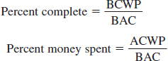
where BAC is the budget at completion.
The program manager uses this information to review the program status with upper-level management. This review is normally on a monthly basis on large projects. In addition, the results of these analyses are used to explain variances in the contractually required reports to the customer.
After the analyses of the variances have been made, reports must be developed for both the customer and in-house (upper-level) management. Customer reporting procedures and specifications can be more detailed than in-house reporting and are often governed by the contract. Contractual requirements specify the reports required, the frequency of submission and distribution, and the customer regulation that specifies the preparation instructions for the report.
The types of reports required by the customer and management depend on the size of the program and the magnitude of the variance. Most reports contain the tracking of the vital technical parameters. These might include:
- The major milestones necessary for project success
- Comparison to specifications
- Types or conditions of testing
- Correlation of technical performance to the activity network and the work breakdown structure
One final note about reports: To save time and money, reports might be only one or two pages or fill-in-the-blank forms.
15.7 THE COST BASELINE
PMBOK® Guide, 4th Edition
7.2.3 Cost Base line
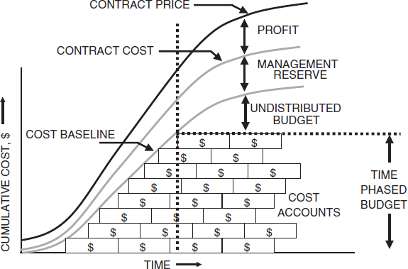
Once the project is initiated, the project team establishes the cost or financial base-line against which status will be reported and variances will be measured. Figure 15-19 represents a cost baseline. Each block represents a cost account or work package element. The summation of all of the cost accounts or work packages would then equal the time-phased budget. Each work package would then be described through the work authorization form for that work package.
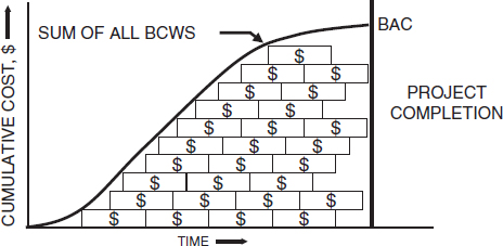
FIGURE 15-19. The cost baseline.
The cost baseline in Figure 15-19 is just part of the cost breakdown. An illustration of a cost breakdown appears in Figure 15-20.
There are certain distinguishing features of Figure 15-20:
- The time-phased budget, which is the released budget, is the summation of all BCWS elements.
- The cost baseline is the summation of the time-phased budget (i.e., the distributed budget) and the undistributed budget. This will equal the released, planned budget at completion (BAC).
- The contractual cost to complete the project is the summation of the cost baseline and the management reserve, assuming that a management reserve exists.
- The contract price is the contract cost plus the profit, if any.
15.8 JUSTIFYING THE COSTS
Project pricing is often based upon best guesses rather than concrete estimates. This is particularly true for companies that survive on competitive bidding and where the preparation cost of a bid may vary between $50,000 and $500,000. If the probability of winning a bid is low, then the company may spend the minimum amount of time and cost during bid preparation.
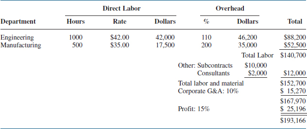
Table 15-7 shows a typical project pricing summary.
In Table 15-7, each functional area or division can have its own overhead rate. In this summary, the overhead rate for engineering is 110 percent, whereas the manufacturing overhead rate is 200 percent. If this company is a subsidiary of a larger company, then a corporate general and administrative (G&A) cost may be included. If the project is for an external customer, then a profit margin will be included.
Once the project pricing summary is completed, the costs must be justified before some executive committee. This is shown in Figure 15-21.
Every company has its own evaluation criteria cost summary approval process. Typical elements that must be justified or supported by hard data include:
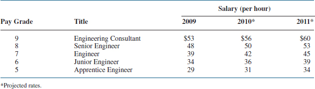
- Labor Rates: For estimating purposes, department averages or skill set weighted averages can be used. This is sometimes called the blended rate. The best-case scenario would be estimating from the actual salary or skill set of the workers to be assigned. This may be impossible during competitive bidding because we do not know who will be available or who will be assigned assuming the contract is received. Also, if the project is a multiyear effort, we may need forward pricing rates, which are the predicted, full burdened salaries anticipated in the next few years. This is illustrated in Table 15-8.
TABLE 15-7. TYPICAL PROJECT PRICING SUMMARY
- Overtime: If resources are scarce and the company has no intention of hiring additional resources, then some of the work must be accomplished on overtime. This could increase the cost of the project and an allowance must be made for possible mistakes made during this period of excessive overtime.
- Scrap Factors: If the project includes procurement of raw materials, then some scrap factor allowance may be necessary. This calculation may be impacted by the skill set of the resources assigned and using the materials, previous experience using these materials, and experience on these types of projects.
TABLE 15-8. FORWARD PRICING RATES: SALARY (Departmental Pay Structure)
- Risks: Risk analysis may be based upon the quality of the estimates and experience of those who made the estimates. Other risks considered include the company's ability to achieve the anticipated benefits or the designated profits and, if a disaster occurs, the company's exposure and liability for lawsuits.
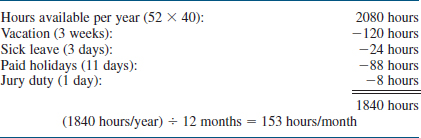
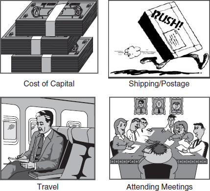
- Hidden Costs: These costs, some of which are illustrated in Figure 15-22, can erode all of the profitability expected on a project. Another potentially hidden cost is the yearly or monthly workload availability. A typical calculation appears in Table 15-9. If we use Table 15-9 and all of the workers are long-term employees, then there may be less than 1840 hours available per year because senior people may have earned more than three weeks of vacation per year.
TABLE 15-9. HOURS AVAILABLE FOR WORK
15.9 THE COST OVERRUN DILEMMA
The lifeblood of most organizations is a continuous stream of new products or services. Because of the word “new,” historical data may be at a minimum and cost overruns are expected. Figure 15-23 shows a typical range of overruns.
Rough order-of-magnitude (ROM) estimates are often made from “soft” data, which can result in a wide range of overruns, and are used in the initiation phase of a project. As we go from soft data to hard data and enter the planning phase of a project, the accuracy of the estimates improves and the range of the overruns narrows.
When overruns occur, the project manager looks for ways of reducing costs. The simplest way is to reduce scope. This begins with a search for items that are easy to cut. The items that are easiest to cut are those items that were poorly understood during the estimating process and were therefore underestimated. Typical items that are cut or reduced in magnitude include:
- Project management supervision
- Line management supervision
- Process controls
- Quality assurance
- Testing
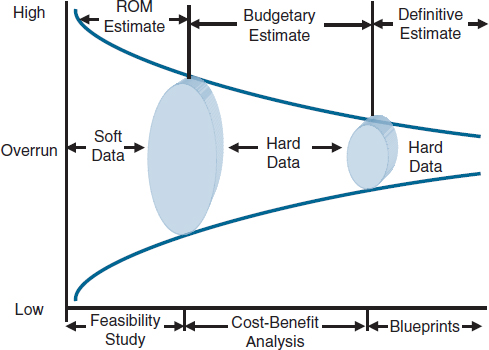
FIGURE 15-23. Range of overruns.
If the easy-to-cut items do not provide sufficient cost reductions, then a desperate search begins among the hard-to-cut items. Hard-to-cut items include:
- Direct labor hours
- Materials
- Equipment
- Facilities
- Others
If the cost reductions are unacceptable to management, then management must decide whether or not to pull the plug and cancel the project. Pulling the plug may seem like an easy decision, but it turns out to be one of the most difficult decisions for executives to make. Typical reasons for not pulling the plug include:
- Quantitative reasons
- High exit barriers
- Significant expenditures have been made and are unrecoverable
- Penalty clauses
- Breach-of-contract lawsuits
- Payments to terminated workers
- Low salvage value of goods and property
- High plant closing costs
- Moving people may end up violating seniority and labor agreements
- Qualitative reasons
- Viewing failure as a sign of weakness
- Viewing failure as damage to one's career
- Viewing failure as damage to one's reputation
- Viewing failure as a roadblock to promotion
- Fear of exposing one's mistakes to others
- Viewing bad news as a personal failure
- Refusing to admit defeat or failure
- Seeing what one wants to see rather than seeing reality
15.10 RECORDING MATERIAL COSTS USING EARNED VALUE MEASUREMENT
Using “earned value” measurement, the actual cost for work performed represents those direct and indirect costs identified specifically for the project (contract) at hand. Both the recorded and reported costs must relate specifically to this effort. Recording direct labor costs usually presents no problem since labor costs are normally recorded as the labor is accomplished. Therefore, recorded and reported labor will be the same.
Material costs, on the other hand, may be recorded at various times. Material costs can be recorded as commitments, expenditures, accruals, and applied costs. All provide useful information and are important for control purposes.
Because of the choices available for material cost analysis, material costs should be reported separately from the standard labor hour/labor dollar earned value report. For example, cost variances associated with the procurement of material may be determined at the time that the purchase orders are negotiated and placed with the vendors since this information provides the earliest visibility of potential cost variance problems. Significant variances in the anticipated and actual costs of materials can have a serious effect on the total contract cost and should be reflected promptly in the estimated cost at completion (EAC) and explained in the narrative part of the project status report.
Separating labor from material costs is essential. Consider the following example:
Example 15-1. You are budgeted to spend $1,000,000 in burdened labor and $600,000 in material. At the end of the first month of your project, the following information is made available to you:
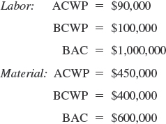
For simplicity's sake, let us use the following formula for EAC:
EAC = (ACWP/BCWP) × BAC
Therefore,
EAC(labor) = $900,000
EAC(material) = $675,000
If we add together both EACs, the estimated cost at completion will be $1,575,000, which is $25,000 below the planned budget. If the costs are combined before we calculate EAC, then
EAC = [($450,000 + $90,000)/$500,000] × ($1,600,000) = $1,728,000
which is a $128,000 overrun. Therefore, it is usually best to separate material from labor in status reporting.
Another major problem is how to account for the costs of material placed on order, which does not reflect the cost of work completed and is not normally used in status reporting. For performance measurement purposes, it is desirable that material costs be recorded at the time that the materials are received, paid for, or used rather than as of the time that they are ordered. Therefore, the actual costs reported for materials should be derived in accordance with established procedures, and normally will be recorded for earned value measurement purposes at or after time of material receipt. In addition, costs should always be recorded on the same basis as budgets are prepared in order to make comparisons between budgeted and actual costs meaningful. For example, material should not be budgeted on the basis of when it is used and then have its costs collected/reported on the basis of when it is received. Consider the following situations:
Situation I: An equipment manufacturer receives a contract to build five machines for the same customer, but each machine is slightly different. The manufacturer purchases and receives five of the same electric motors, one for each machine. What is the earliest time that the manufacturer should take credit for the electric motors?
- When ordered
- When received
- When paid for
- When withdrawn from inventory
- When installed
Situation II: The same manufacturer has purchased large quantities of steel plate for the five machines as well as for machines for other customers. By ordering in large quantities, the manufacturer received a substantial price break. What is the earliest time the manufacturer should take credit for the steel plate?
- When ordered
- When received
- When paid for
- When withdrawn from inventory
- When installed
Situation III: Assume that the manufacturer in Situation II purchases the steel plate for a single customer rather than for multiple customers. What is the earliest time the manufacturer should take credit for the steel plate?
- When ordered
- When paid for
- When received
- When applied
In Situations I and III, the recommended answer is “when received.” In Situation II, any answer can be argued, but the preferred answer is “when installed.”
15.11 THE MATERIAL ACCOUNTING CRITERION7
At a minimum, the contractor's material accounting system must provide for the following:
- Accurate cost accumulation and assignment of costs to cost accounts in a manner consistent with budgets using recognized, acceptable costing techniques.
- Determination of material price variances by comparing planned versus actual commitments.
- Cost performance measurement at the point in time most suitable for the category of material involved, but no earlier than the time of actual receipt of material.
- Determination of material cost variances attributable to the excess usage of material.
- Determination of unit or lot costs when applicable.
- Full accountability for all material purchased for the project, including residual inventory.
In order to satisfy these six system requirements, the following accounting practices should be adhered to:
- The material cost actuals (ACWP) must equate to its material plans (BCWS), and be carried down to the cost account level of the WBS.
- The material price variances must be determinable by comparing planned commitments (estimated material value) to actual commitments (actual cost of the material).
- Physical work progress or earned value (BCWP) must be determinable, but not before the materials have been received.
- Usage cost variances (to be discussed in the next section) must be determinable from excess material usage.
- Material unit costs and/or lot costs must be determinable, as applicable.
- There must be full accountability of all materials purchased, including any residual material inventory.
Although this task appears difficult on the surface, it is easy if the organization focuses on two areas:
- The material plans (BCWS): These frequently start at the point at which engineering or manufacturing or others have provided a definition sufficient to initiate an order for the items, regardless of when such items are actually ordered or received.
- The material actuals (ACWP): This is ordinarily the point at which the costs of the parts are recorded on the firm's accounting books, that is, when the bill is paid.
Those firms that have a material commitment system in use as part of the material accounting system are usually able to establish and update the costs for their purchased goods at multiple points: as an estimated liability when engineering or manufacturing defines the requirements; still as an estimated liability when someone formally initiates the request; updated to an accrued liability when an order is placed by purchasing; later updated to an actual liability when parts are received and accepted; and updated a final time when the bill is paid and the costs are recorded on the accounting books.
15.12 MATERIAL VARIANCES: PRICE AND USAGE8
One of the requirements of a material accounting system is that it be able to determine just why material budgets were exceeded; this is called variance analysis. When the actual material costs exceed a material budget, there are normally two causes:
- The articles purchased cost more than was planned, called a “price variance.”
- More articles were consumed than were planned, called a “usage variance.”
Price variances (PV) occur when the budgeted price value (BCWS) of the material was different than what was actually experienced (ACWP). This condition can arise for a host of reasons: poor initial estimates, inflation, different materials used than were planned, too little money available to budget, and so on.
The formula for price variance (PV) is:
PV = (Budgeted price − Actual price) × (Actual quantity)
Price variance is the difference between the budgeted cost for the bill of materials and the price paid for the bill of materials.
By contrast, usage variances (UV) occur when a greater quantity of materials is consumed than were planned. The formula for usage variance (UV) is:
UV = (Budgeted quantity − Actual quantity) × (Budgeted price)
Normally, usage variances are the resulting costs of materials used over and above the quantity called for in the bill of materials.
Consider the following example: The project manager establishes a material budget of 100 units (which includes 10 units for scrap factor) at a price of $150 per unit. Therefore, the material budget was set at $15,000. At the end of the short project, material actuals (ACWP) came in at $15,950, which was $950 over budget. What happened?
Applying the formulas defined previously,
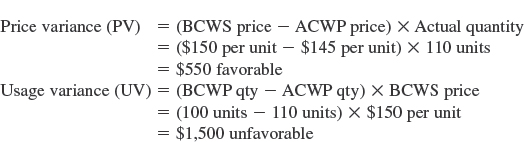
The analysis indicates that your purchase price was less than you anticipated, thus generating a cost savings. However, you used 10 units more than planned for, thus generating an unfavorable usage variance. Further investigation indicated that your line manager had increased the scrap factor from 10 to 20 units.
Good business practices indicate that such variance analyses take place to determine why actual material costs exceed the budgeted material values.
15.13 SUMMARY VARIANCES
Summary variances can be calculated for both labor and material. Consider the information shown below:
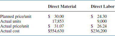
We can now calculate the total price variance for direct material and the rate cost variance:
- Total price variance for direct material
= Actual units × (BCWP − ACWP)
= 17,853 × ($30.00 − $31.07)
= $19,102.71 (unfavorable)
- Labor rate cost variance
= Budgeted rate × Actual rate
= $24.30 × $26.24
= $1.94 (unfavorable)
15.14 STATUS REPORTING
PMBOK® Guide, 4th Edition
10.5.3.1 Performance Reporting
One of the best ways of reducing executive meddling on projects is to provide executives with frequent, meaningful status reports. Figure 15-24 shows a relatively simple status report based upon data accumulation in the form of Figures 15-25 and 15-26. These types of status reports should be short and concise, containing pertinent information only. Status can also be shown graphically as in Figure 15-27. The difference between Figure 15-27 and 15-17 is that at-completion estimates have been identified.
As the available project management software becomes more sophisticated, so does project reporting. There are four types of reports that are generally printed out from the earned value measurement system:
- Performance Reports: These reports indicate the physical progress to date, namely, BCWS, BCWP, and ACWP. The report might also include information on material procurement, delivery, and usage, but most companies have separate reports on materials.
- Status Reports: These reports identify where we are today and use the information from the performance reports to calculate SV and CV.
- Projection Reports: These reports calculate EAC, ETC, SPI, and CPI as well as any other forward-looking projections. These reports emphasize where we will end up.
- Exception Reports: These reports identify exceptions, problems, or situations that exceed the threshold limits on such items as variances, cash flow, resources assigned, and other such topics.
Reporting procedures for variance analysis should be as brief as possible. The reason for this is simple: the shorter and more concise the report, the faster that feedback can be generated and responses developed. Time is critical if rescheduling must be accomplished with limited resources. The two most common situations providing constraints on resource rescheduling are that:
- The end date is fixed
- The resources available are constant (or limited)
With a fixed end date, program rescheduling generally requires that additional resources be supplied. In the second situation, program slippage may be the only alternative unless a constant stream of resources can be redistributed so as to shorten the length of the critical path.
Once the variance analysis is completed, both project and functional management must diagnose the problem and search for corrective actions. This includes:
- Finding the cure for the problem
- Developing a plan to recover the position
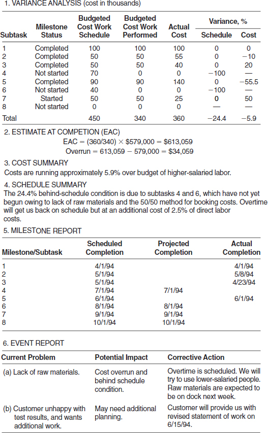
FIGURE 15-24. Blue Spider Project, monthly project report #4.
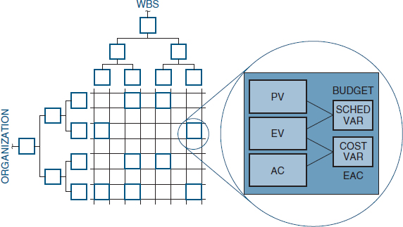
FIGURE 15-25. Data accumulation.
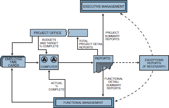
FIGURE 15-26. Cost control and report flow.
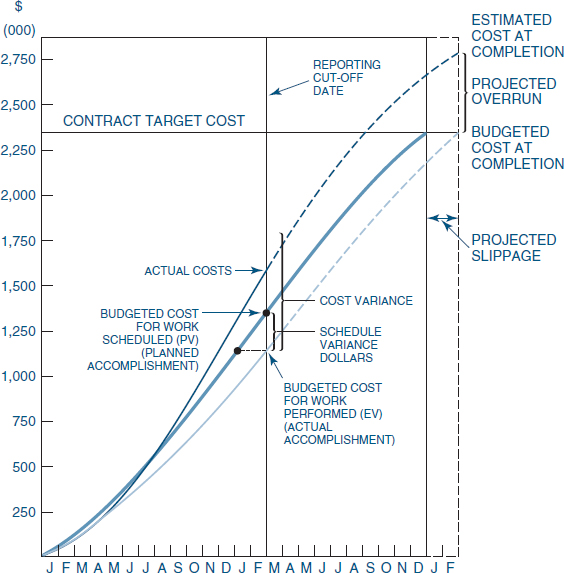
FIGURE 15-27. Graphical status reporting.
This by no means implies that all variances require corrective action. There are four major responses to a variance report:
- Ignoring it
- Functional modification
- Replanning
- System redesign
Permissible variances exist for all levels of the organization. If the variance is within these permitted deviations, then there will be no response, and the variance may be ignored. In some situations where the variance is marginal (or even within limits), corrective action may be required. This would normally occur at the functional level and might simply involve using another test procedure or possibly considering some alternative not delineated in the program plan.
If major variances occur, then either replanning or system redesign must take place. The replanning process requires the redefining and reestablishing of project goals as work progresses, but always within system specifications. This might include making trade-offs in time, cost, and performance or defining new project activities and methods of pursuing the project, such as new PERT networks. If resources are limited, then a proper redistribution or reallocation must be made. If resources are not limited, the additional personnel, financing, equipment, facilities, or information may be required.
If replanning cannot be accomplished without system redesign, then system specifications may have to be changed.9 This is the worst possible case because performance may be sacrificed to satisfy the constraints of time and money.
Whenever companies operate on a matrix structure, information must be carefully prepared and distributed to all key individuals in the organization. To avoid dual standards and red tape, management must establish the decision-making policies associated with cost and control systems. The following is a policy guide:
- Approving all estimates, and negotiating all estimates and the definition of work requirements with the respective organizations.
- Approving the budget, and directing distribution and budgeting of available funds to all organizational levels by program element.
- Defining the work required and the schedule.
- Authorizing work release. The manager may not, however, authorize work beyond the scope of the contract.
- Approving the program bill-of-materials, detailed plans, and program schedules for need and compliance with program requirements.
- Approving the procuring work statement, the schedules, the source selection, the negotiated price, and the type of contract on major procurement.
- Monitoring the functional organization's performance against released budgets, schedules, and program requirements.
- When cost performance is unacceptable, taking appropriate action with the affected organization to modify the work requirements or to stimulate corrective action within the functional organization so as to reduce cost without changing the contracted scope of work.
- Being responsible for all communications and policy matters on contracted programs so that no communicative directives shall be issued without the signature or concurrence of the program manager.
TABLE 15-10. PROGRAM INTERRELATIONSHIPS
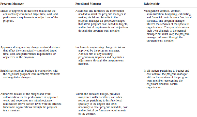
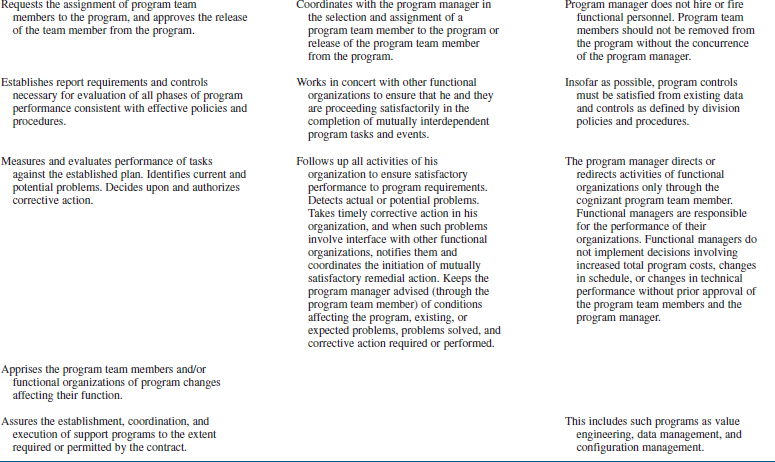
Describing the responsibilities of a manager is only a portion of the management policy. Because the program manager must cross over functional boundaries to accomplish all of the above, it is also necessary to describe the responsibilities of the functional manager and the relationship between the two. Table 15-10 is an example of this. Similar tables can be developed for planning and scheduling, communications, customer relations, and contract administration.
15.15 COST CONTROL PROBLEMS
PMBOK® Guide, 4th Edition
7.3 Cost Control
No matter how good the cost and control system is, problems can occur. Common causes of cost problem include:
- Poor estimating techniques and/or standards, resulting in unrealistic budgets
- Out-of-sequence starting and completion of activities and events
- Inadequate work breakdown structure
- No management policy on reporting and control practices
- Poor work definition at the lower levels of the organization
- Management reducing budgets or bids to be competitive or to eliminate “fat”
- Inadequent formal planning that results in unnoticed, or often uncontrolled, increases in scope of effort
- Poor comparison of actual and planned costs
- Comparison of actual and planned costs at the wrong level of management
- Unforeseen technical problems
- Schedule delays that require overtime or idle time costing
- Material escalation factors that are unrealistic
Cost overruns can occur in any phase of project development. The most common causes for cost overruns are:
- Proposal phase
- Failure to understand customer requirements
- Unrealistic appraisal of in-house capabilities
- Underestimating time requirements
- Planning phase
- Omissions
- Inaccuracy of the work breakdown structure
- Misinterpretation of information
- Use of wrong estimating techniques
- Failure to identify and concentrate on major cost elements
- Failure to assess and provide for risks
- Negotiation phase
- Forcing a speedy compromise
- Procurement ceiling costs
- Negotiation team that must “win this one”
- Contractual phase
- Contractual discrepancies
- SOW different from RFP requirements
- Proposal team different from project team
- Design phase
- Accepting customer requests without management approval
- Problems in customer communications channels and data items
- Problems in design review meetings
- Production phase
- Excessive material costs
- Specifications that are not acceptable
- Manufacturing and engineering disagreement
15.16 STUDYING TIPS FOR THE PMI® PROJECT MANAGEMENT CERTIFICATION EXAM
This section is applicable as a review of the principles to support the knowledge areas and domain groups in the PMBOK® Guide. This chapter addresses:
- Scope Management
- Cost Management
- Initiating
- Planning
- Controlling
Understanding the following principles is beneficial if the reader is using this text to study for the PMP® Certification Exam:
- What is meant by a management cost and control system
- What is meant by earned value measurement
- The meaning of control
- Code of cost accounts
- Work authorization for and its relationship to the code of accounts
- Sources of funds for a project or changes to a project
- Four primary elements of cost monitoring and control: BCWS, BCWP, ACWP, and BAC
- How to calculate the cost and schedule variances, in hours, dollars, and percentages
- Importance of SPI and CPI in trend analysis
- Ways to forecast the time and cost to completion as well as variances at completion
- Different types of reports: performance, status, forecasting, and exception
- Use of the management reserve
- Escalation factors and how they affect a project
- What is a cost or financial baseline for a project
- Different ways to calculate either BCWP or percent complete
The following multiple-choice questions will be helpful in reviewing the principles of this chapter:
- In earned value measurement, earned value is represented by:
- BCWS
- BCWP
- ACWP
- None of the above
- If BCWS = 1000, BCWP = 1200, and ACWP = 1300, the project is:
- Ahead of schedule and under budget
- Ahead of schedule and over budget
- Behind schedule and over budget
- Behind schedule and under budget
- If BAC = $20,000 and the project is 40 percent complete, then the earned value is:
- $5000
- $8000
- $20,000
- Cannot be determined
- If BAC = $12,000 and CPI = 1.2, then the variance at completion is:
- −$2000
- +$2000
- −$3000
- +$3000
- If BAC = $12,000 and CPI = 0.8, then the variance at completion is:
- −$2000
- +$2000
- −$3000
- +$3000
- If BAC for a work package is $10,000 and BCWP = $4,000, then the work package is:
- 40 percent complete
- 80 percent complete
- 100 percent complete
- 120 percent complete
- If CPI = 1.1 and SPI = 0.95, then the trend for the project is:
- Running over budget but ahead of schedule
- Running over budget but behind schedule
- Running under budget but ahead of schedule
- Running under budget but behind schedule
- The document that describes a work package, identifies the cost centers allowed to charge against this work package, and establishes the charge number for this work package is the:
- Code of accounts
- Work breakdown structure
- Work authorization form
- None of the above
- Unknown problems such as escalation factors are often budgeted for using the:
- Project manager's charge number
- Project sponsor's charge number
- Management reserve
- Configuration management cost account
- EAC, ETC, SPI, and CPI most often appear in which type of report?
- Performance
- Status
- Forecast
- Exception
- If BAC = $24,000, BCWP = 12,000, ACWP = $10,000, and CPI = 1.2, then the cost that remains to finish the project is:
- $10,000
- $12,000
- $14,000
- Cannot be determined
- There are several purposes for the 50–50 rule, but the primary purpose of the 50-50 rule is to calculate:
- BCWS
- BCWP
- ACWP
- BAC
- When a project is completed, which of the following must be true?
- BAC = ACWP
- ACWP = BCWP
- SV = 0
- BAC = ETC
- In March CV = −$20,000, and in April CV = −$30,000. In order to determine whether or not the situation has really deteriorated because of a larger unfavorable cost variance, we would need to calculate:
- CV in percent
- SV in dollars
- SV in percent
- All of the above
- If a project manager is looking for revenue for a value-added scope change, the project manager's first choice would be:
- Management reserve
- Customer-funded scope change
- Undistributed budget
- Retained profits
- A project was originally scheduled for 20 months. If CPI is 1.25, then the new schedule date is:
- 16 months
- 20 months
- 25 months
- Cannot be determined
- The cost or financial baseline of a project is composed of:
- Distributed budget only
- Distributed and undistributed budgets only
- Distributed budget, undistributed budget, and the management reserve only
- Distributed budget, undistributed budget, management reserve, and profit only
ANSWERS
- B
- B
- B
- B
- C
- A
- D
- C
- C
- C
- A
- B
- C
- A
- B
- D
- B
PROBLEMS
15–1 Do cost overruns just happen, or are they caused?
15–2 Cemeteries are filled with projects that went out of control. Below are several causes that can easily develop into out-of-control conditions. In which phase of a project should each of these conditions be detected and, if possible, remedied?
- Customer's requirements not understood
- Project team formed after bid was prepared
- Accepting unusual terms and conditions
- Permitting a grace period for changing specifications
- Lack of time to research specifications
- Overestimation of company's capabilities
15–3 Below are several factors that can result in project delays and cost overruns. Explain how these problems can be overcome.
- Poorly defined milestones
- Poor estimating techniques
- A missing PERT/CPM chart
- Functional managers not having a clear understanding of what has to be done
- Poor programming procedures and techniques
- Changes constantly being made deep in the project's life cycle
15–4 Under what circumstances would each of the figures in Chapter 13 be applicable for customer reporting? In-house reporting? Reporting to top-level management?
15–5 What impact would there be on BCWS, BCWP, ACWP, and cost and schedule variances as a result of the:
- Early start of an activity on a PERT chart?
- Late start of an activity on a PERT chart?
15–6 Alpha Company has implemented a plan whereby functional managers will be held totally responsible for all cost overruns against their (the functional managers') original estimates. Furthermore, all cost overruns must come out of the functional managers' budgets, whether they be overhead or otherwise, not the project budget. What are the advantages and disadvantages of this approach?
15–7 Karl has decided to retain a management reserve on a $400,000 project that includes a $60,000 profit. At the completion of the project, Karl finds that the management reserve fund contains $40,000. Should Karl book the management reserve as excess profits (i.e., $100,000), or should he just book the target profit of $60,000 and let the functional managers “sandbag” on the slush fund until it is depleted?
15–8 ABC Corporation has recently given out a nine-month contract to a construction subcontractor. At the end of the first month, it becomes obvious that the subcontractor is not reporting costs according to an appropriate WBS level. ABC Corporation asks the subcontractor to change its cost reporting procedures. The subcontractor states that this cannot be done without additional funding. This problem has occurred with other subcontractors as well. What can ABC Corporation do about this?
15–9 What would be the result if all project managers decided to withhold a management reserve? What criteria should be used for determining when a management reserve is necessary?
15–10 Alpha Company, a project-driven organization, pays its department managers a quarterly bonus that is dependent on two factors: the departmental overhead rate and direct labor dollars. The exact value of the bonus is proportional to how much these two factors are underrun.
Department man-hours are priced out against the department average, which does not include the department manager's salary. His salary is included under his departmental overhead rate, but he does have the option of charging his own time as direct labor to the projects for which he must supply resources.
What do you think of this method? Is it adequate inducement for a functional manager to control resources more effectively? How would you feel, as a project manager, knowing that the functional managers got quarterly bonuses and you got none?
15–11 Many executives are reluctant to let project managers have complete control of project costs because then the project managers must know the exact salaries of almost all project personnel. Can this situation be prevented if the contract requires reporting costs as actuals?
15–12 How can a country's inflation rate influence the contractual payment policy?
15–13 Consider a situation in which several tasks may be for one to two years rather than the 200 hours normally used in the work-package level of the WBS.
- How will this affect cost control?
- Can we still use the 50/50 rule?
- How frequently should costs be updated?
15–14 By now you should be familiar with the various tools that can be used for planning, controlling, scheduling, and directing project activities. Table 15-11 contains a partial list of such tools and how they relate to specific project management functions. Complete the table (using the legend at the bottom) to indicate which are very useful and which are somewhat useful.
Obviously there will be some questions about what is very useful and what is somewhat useful. Be able to defend your answers.
TABLE 15-11. PROJECT PLANNING, CONTROLLING, AND DIRECTING
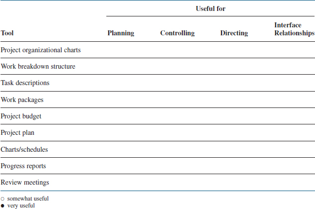
15–15 Complete the table below and plot the EAC as a function of time. What are your conclusions?
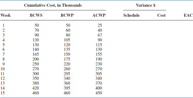
15–16 Using the information in Chapter 12, problem 12-18, complete Table 15-12.
15–17 On June 12, 2002, Delta Corporation was awarded a $160,000 contract for testing a product. The contract consisted of $143,000 for labor and materials, and the remaining $17,000 was profit. The contract had a scheduled start date of July 3. The network logic, as defined by the project manager and approved by the customer, consisted of the following:
| Activity | Time (Weeks) |
| AB | 7 |
| AC | 10 |
| AD | 8 |
| BC | 4 |
| BE | 2 |
| CF | 3 |
| DF | 5 |
| EF | 2 |
| FG | 1 |
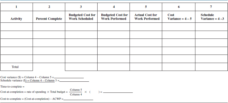
On August 27, 2002, the executive steering committee received the following report indicating the status of the project at the end of the eighth week:
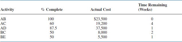
The steering committee could not identify the real status of the project from this brief report. Even after comparing this brief status report with the project planning budget (see Table 15-13), the real status was not readily apparent.
Management instructed the project manager to prepare a better status report that depicted the true status of the project, as well as the amount of profit that could be expected at project completion. Your assignment is to prepare a table such as Table 15-12.
15–18 The Alpha Machine Tool Project
Acme Corporation has received a contractual order to build a new tooling machine for Alpha Corporation. The project started several months ago. Table 15-14 is the Monthly Cost Summary for June, 2002. Some of the entries in the table have been purposely omitted, but the following additional information is provided to help you answer the questions below:
- Assume that the overhead of 100% is fixed over the period of performance.
- The report you are given is at a month end, June 30, 2002.
- The 80/20 sharing ratio says that the customer (i.e., Alpha) will pay 80 percent of the dollars above the target cost and up to the ceiling cost. Likewise, 80 percent of the cost savings below the target cost go back to Alpha.
- The revised BCWS is revised from the released BCWS.
- The ceiling price is based on cost (i.e., without profit).
Answer the following questions by extracting data from the Alpha Machine Tool Project's monthly summary report.
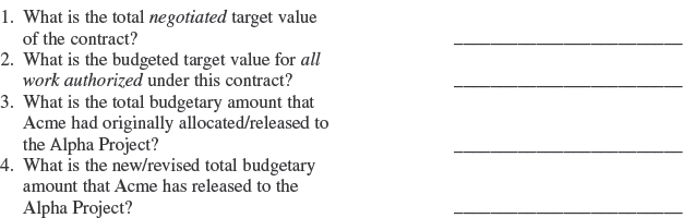
TABLE 15-13. PROJECT PLANNING BUDGET
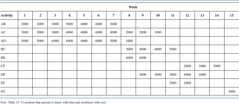
TABLE 15-14. MONTHLY COST SUMMARY—JUNE 2002
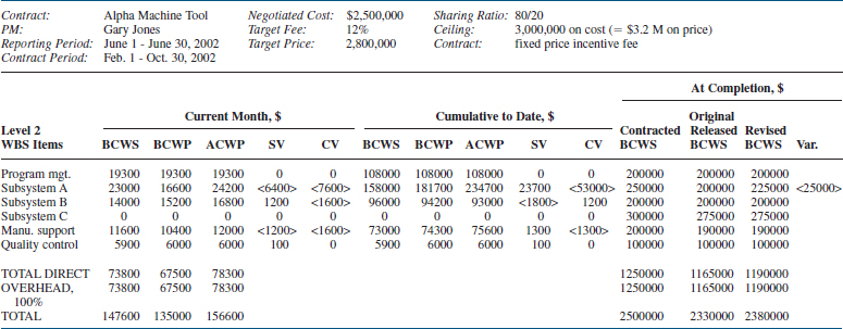
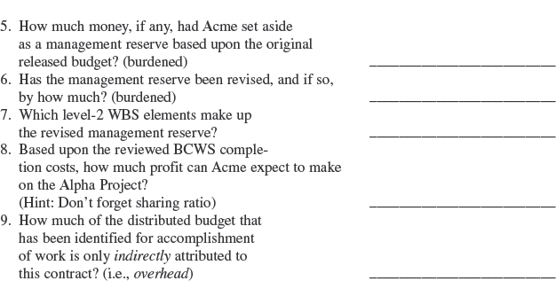
Answer the Following Questions for Direct Labor Only
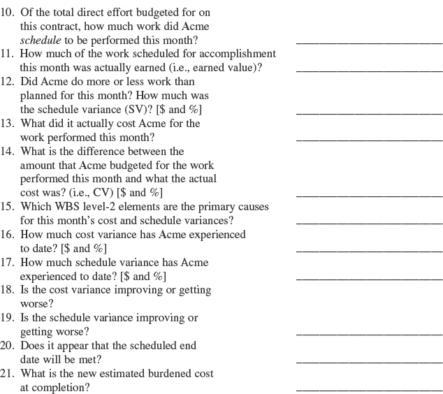
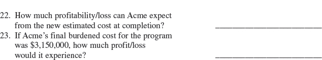
15–19 Calculate the total price variance for direct labor and the labor rate cost variance from the following data:
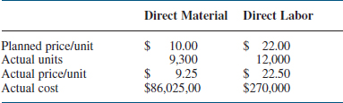
15–20 One of your assistant project managers has given you an earned value report that is only partially complete. Can you fill in the missing information?
(All numbers are in thousands of dollars)
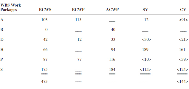
15–21 The following problem requires an understanding of the WBS, the cost account elements, and cost control analysis. Assume that all costs are in thousands of dollars.
Given the partial WBS shown below, what is the total cost for the WBS element 4.0? Assume that the costs provided are direct labors costs only and that the overhead rate is 100 percent.
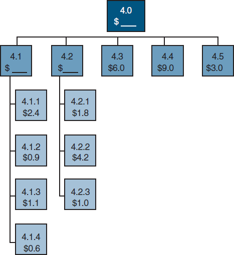
Which of the following is the value of WBS element 4.0?
- $60.0
- $30.0
- $24.0
- $54.0
Using the data in Figure 15-28, and the actual costs given below for WBS elements 5.1 through 5.4 and elements 4.1 and 4.2, answer the questions shown below:
| Actual Costs | |
| E-1-5.1 | $1.0 |
| E-1-5.3 | $1.5 |
| E-2-5.2 | $1.0 |
| E-2-5.4 | $2.0 |
| E-3-5.1 | $1.0 |
| E-3-5.3 | $2.5 |
| E-4-5.3 | $3.0 |
| E-4-5.2 | $3.5 |
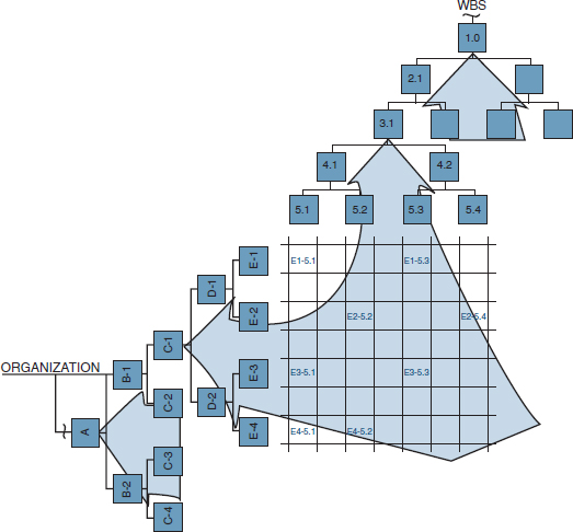
FIGURE 15-28. Exhibit of cost accounts.
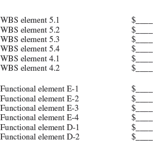
15–22 Companies usually estimate work based upon man-months. If the work must be estimated in man-weeks, the man-month is then converted to man-weeks. The problem is in the determination of how many man-hours per month are actually available for actual direct labor work.
Your company has received a request for proposal (RFP) from one of your customers and management has decided to submit a bid. Only one department in your company will be required to perform the work and the department manager estimates that 3000 hours of direct labor will be required.
Your first step is to calculate the number of hours available in a typical man-month. The Human Resources Department provides you with the following yearly history for the average employee in the company:
- Vacation (3 weeks)
- Sick days (4 days)
- Paid holidays (10 days)
- Jury duty (1 day)
- How many direct labor hours are available per month per person?
- If only one employee can be assigned to the project, what will be the duration of the effort, in months?
- If the customer wants the job completed within one year, how many employees should be assigned?
15–23 In a status report, executives want to know not only where we are today, but also where we will end up. Calculating where we will end up financially is not as easy as it sounds. Selecting the wrong formula can leave the executives and customers with a faulty impression.
There are several formulas available for the calculation of the estimated cost at completion (EAC). For simplicity, consider the following three formulas:
- EAC = (ACWP/BCWP) × (budget at completion)
- EAC = [(ACWP/BCWP) × (BCWS for work completed and in progress)] + (planned or revised planned costs of work packages not yet begun)
- EAC = (actual to date) + (all remaining work, including work in progress, to be completed at the planned or budgeted costs)
- Using the table below, determine the value of EAC for each of the three formulas. Assume that A, B, and C are the only work packages in the project, and BCWS(Total) is the total value for PV for each work package rather than PV for the reporting period. Use the following formula for calculating EV:
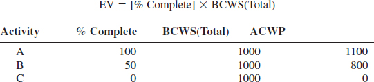
- Considering only activity B, if the reason for the cost overrun is attributed to a one-time occurrence, which of the three formulas would be best to use?
- If the reason for the overrun in activity B is because of the higher than expected salaries of the assigned employees and these same employees will be assigned to activity C as well, which of the three formulas would be best to use?
- Considering only activity B, if the reason for the overrun is attributed to overtime and the overtime will continue but only through the completion of activity B, which of the three formulas would be best to use?
- Considering your answers to the above four parts, should a company be willing to change the formula for calculating EAC during the execution of the project as well as at each reporting period or gate review meeting?
- Using the table below, determine the value of EAC for each of the three formulas. Assume that A, B, and C are the only work packages in the project, and BCWS(Total) is the total value for PV for each work package rather than PV for the reporting period. Use the following formula for calculating EV:
15–24 Project managers must not only calculate variances but also determine the root cause of the variance. Some variances may be allowable while others must be explained together with a corrective plan for recovery.
In the table below, you must demonstrate your ability to calculate the cost and schedule variances as well as determine the root cause of the variances, if possible. Consider the following table, which shows a partial status report for a project composed of five work packages (i.e., activities):
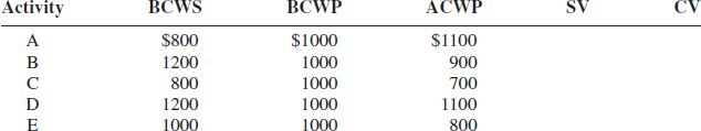
- Calculate the cost and schedule variances, in dollars, for each activity.
- For each activity, which of the following could be the root cause reason for the variances? Select as many as you think may apply.
- Accelerated schedule due to higher salaried personnel
- Accelerated schedule due to overlapping of activities
- Accelerated schedule due to overtime
- Accelerated schedule due to additional resources
- Slippage due to lack of resources
- Slippage due to people working on other projects
- Slippage due to mistakes
- People are working but progress is poor
- On schedule
- On budget
- Over budget
- Management wants to know the status of the total project at level 1 of the WBS. Add up all of the activity cost and schedule variances to determine the level 1 cost and schedule variances. What are your conclusions?
- Would your conclusions from part c above change if activities B and D were the only two activities on the critical path?
15–25 Sometimes, the root cause of a variance requires that variance analysis be performed in both hours and dollars. It is possible that calculating the variances in both hours and dollars is the only way to determine the root cause of a problem.
Problem: In Table 15-15, the cost and schedule variances are measured in fully burdened dollars for Cost Center 2834 only.
From Table 15-15, you are ahead of schedule and over budget. There could be several possible causes for this, including schedule compression, using higher salaried labor, overtime, additional resources, or other causes. How can we determine which of these causes is the real reason for the variances?
Table 15-16 shows the variance data in both hours and dollars.
- Calculate the cost variances in both hours and dollars. Compare the results. What are your conclusions?
- Calculate the planned fully burdened labor rate using BCWS (or BCWP).
- Calculate the actual fully burdened labor rate using ACWP.
- Explain the possible reasons for the differences in labor rates and how this affects your answer to part a.
- Table 15-17 shows the departmental pay structure for Cost Center 2834. Determine the departmental overhead rate, in percent.
- How does Table 15-17 affect your answer to part d?
TABLE 15-15. COST CENTER 2834, JUNE
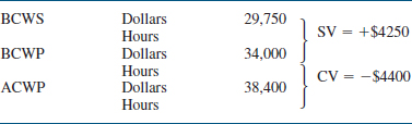
TABLE 15-16. COST CENTER 2834, JUNE
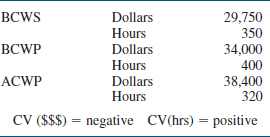
TABLE 15-17. DEPARTMENTAL PAY STRUCTURE
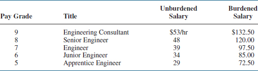
15–26 Projects that span more than one year or cut across the date of corporate salary increases may require the use of forward-pricing rates. Forward-pricing rates are determined from economic data, industry surveys, and best-guess predictions.
As an example, consider Table 15-17 in the previous problem, which shows the salary structure for an engineering department. For simplicity, we shall make the following assumptions:
- Promotions and salary increases, including cost-of-living adjustments, are effective January 1 and are then held constant for the entire year.
- The overhead rate is 150 percent and fixed for the entire year.
- All projects are priced out using the salary of a pay grade 7.
- Most of the departmental workers are pay grade 7 employees.
Situation: Your company has just won a one-year contract. The contract was planned to start on January 1, 2006, and be completed by December 31, 2006. The work that was to be performed by this department was estimated at 1000 hours per month for the duration of the twelve-month project using pay grade 7 employees. The customer informs you that they wish to start the project on July 1 rather than January 1, and they assume that there is no financial impact on the total cost of the project.
The Finance Department provides you with the forward pricing rate data in Table 15-18 and tells you that the overhead rate for 2007 is expected to increase to 155 percent. Is there a financial impact on the total cost of the project, and if so, how much of an impact?
TABLE 15-18. DEPARTMENTAL PAY STRUCTURE (dollars/hour)
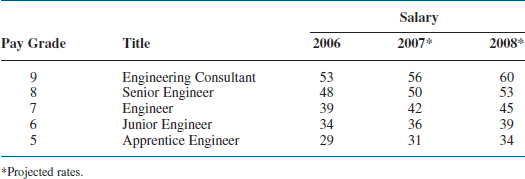
TABLE 15-19. PROJECT PRICING SUMMARY
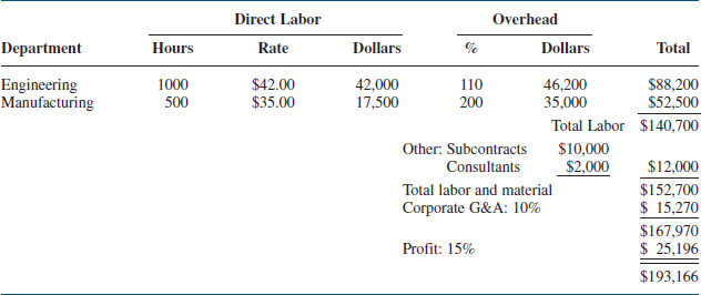
15–27 Pricing out a customer's request for proposal is a trade-off between time, cost, and accuracy. If time and money are not an issue, then we could determine a very accurate bid. But if the company is reluctant to invest heavily in the preparation of the bid, care must be taken that there are no hidden costs.
Situation: You have been asked to price out a project for a customer, and this pricing is an activity with which you have very little previous experience. Table 15-19 shows the numbers that you arrived at in determining that a bid of $193,166 should be submitted.
Before a bid is submitted to a potential customer, the bid must be reviewed by a committee of senior managers that can question the validity of the numbers as well as look for “hidden” costs that may have been omitted. For each of the situations below, which line item in the pricing summary would most likely be impacted assuming that these hidden costs were not already included?
- Management tells you that, during the execution of the project, the customer will want three interface meetings with the customer held at the customer's location. The Travel Group within your company informs you that airfare, ground travel, meals, and lodging are expected to be approximately $2000 per meeting.
- One of the executives comments, “The shipping costs for the deliverables, including insurance, packaging, and handling, will be about $1000. I do not see this included in your summary.”
- The RPF for the project stated that the contract would be firm-fixed-price with a lump-sum payment at the end of the project after approval/acceptance of the final deliverables. The cost of capital is expected to be approximately $6000.
- Engineering believes that the engineering hours in the summary could be low by about 10 percent if the risks in the estimates provided actually occur. The executives believe that a management reserve of 10 percent should be included in the summary costs.
- Using the information in parts a through d above, what final price should be submitted to the customer?
15–28 A homeowner hires a contractor to build a four-sided square fence around his home. The homeowner provides the materials and the contractor supplies the labor. The contractor estimates each side will cost $2000 and require one week in duration.
At the end of week 1, the first side is completed at a cost of $2000. During week 2, the second side is completed but at a cost of $2400 because the contractor damaged a water line that the contractor had to repair. During week 3, the contractor completed only half of the fence for $1000 because it rained for the remaining half of the week.
At the end of week 3, the contractor must prepare an earned value measurement status report. Calculate the following:
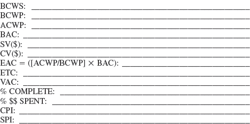
15–29 The data identified below was listed in a project's latest status report:
- BCWS = $36,000
- BCWP = $30,000
- ACWP = $33,000
- BAC = $120,000
- Original length of the project 10 months
Using these data, calculate the following:
- What are the values for CPI and SPI?
- What is the expected cost at completion (EAC)?
- How much money will be needed from the time of the report to complete the project?
- What is the cost variance at completion (VAC)?
- Using SPI, what is the new expected length of the project?
15–30 In the problem in Figure P15-30, the 50% / 50% rule is being used to determine the project's status. Assume that all amounts are in dollars.
Assuming that ACWP = $40,000, determine BCWS, BCWP, BAC, SV, and CV.
15–31 In Figures P15–31A to P15–31C identify the status of part of a project using the graphical technique (i.e. S curves) rather that tables. For each of the three figures, select from one of the following fives choices as to what each figure illustrates:
- Over budget
- Under budget
- Ahead of schedule
- Behind schedule
- Status cannot be determined
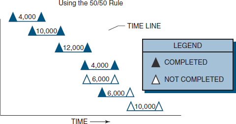
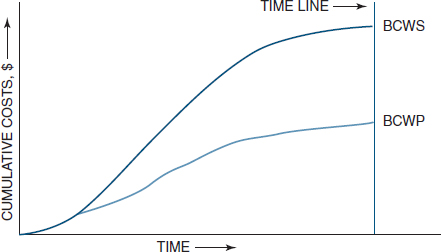
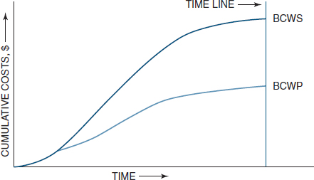
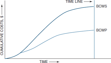
CASE STUDIES
THE BATHTUB PERIOD
The award of the Scott contract on January 3, 1987, left Park Industries elated. The Scott Project, if managed correctly, offered tremendous opportunities for follow-on work over the next several years. Park's management considered the Scott Project as strategic in nature.
The Scott Project was a ten-month endeavor to develop a new product for Scott Corporation. Scott informed Park Industries that sole-source production contracts would follow, for at least five years, assuming that the initial R&D effort proved satisfactory. All follow-on contracts were to be negotiated on a year-to-year basis.
Jerry Dunlap was selected as project manager. Although he was young and eager, he understood the importance of the effort for future growth of the company. Dunlap was given some of the best employees to fill out his project office as part of Park's matrix organization. The Scott Project maintained a project office of seven full-time people, including Dunlap, throughout the duration of the project. In addition, eight people from the functional department were selected for representation as functional project team members, four full-time and four half-time.
Although the workload fluctuated, the manpower level for the project office and team members was constant for the duration of the project at 2,080 hours per month. The company assumed that each hour worked incurred a cost of $60.00 per person, fully burdened.
At the end of June, with four months remaining on the project, Scott Corporation informed Park Industries that, owing to a projected cash flow problem, follow-on work would not be awarded until the first week in March (1988). This posed a tremendous problem for Jerry Dunlap because he did not wish to break up the project office. If he permitted his key people to be assigned to other projects, there would be no guarantee that he could get them back at the beginning of the follow-on work. Good project office personnel are always in demand.
Jerry estimated that he needed $40,000 per month during the “bathtub” period to support and maintain his key people. Fortunately, the bathtub period fell over Christmas and New Year's, a time when the plant would be shut down for seventeen days. Between the vacation days that his key employees would be taking, and the small special projects that his people could be temporarily assigned to on other programs, Jerry revised his estimate to $125,000 for the entire bathtub period.
At the weekly team meeting, Jerry told the program team members that they would have to “tighten their belts” in order to establish a management reserve of $125,000. The project team understood the necessity for this action and began rescheduling and replanning until a management reserve of this size could be realized. Because the contract was firm-fixed-price, all schedules for administrative support (i.e., project office and project team members) were extended through February 28 on the supposition that this additional time was needed for final cost data accountability and program report documentation.
Jerry informed his boss, Frank Howard, the division head for project management, as to the problems with the bathtub period. Frank was the intermediary between Jerry and the general manager. Frank agreed with Jerry's approach to the problem and requested to be kept informed.
On September 15, Frank told Jerry that he wanted to “book” the management reserve of $125,000 as excess profit since it would influence his (Frank's) Christmas bonus. Frank and Jerry argued for a while, with Frank constantly saying, “Don't worry! You'll get your key people back. I'll see to that. But I want those uncommitted funds recorded as profit and the program closed out by November 1.”
Jerry was furious with Frank's lack of interest in maintaining the current organizational membership.
- Should Jerry go to the general manager?
- Should the key people be supported on overhead?
- If this were a cost-plus program, would you consider approaching the customer with your problem in hopes of relief?
- If you were the customer of this cost-plus program, what would your response be for additional funds for the bathtub period, assuming cost overrun?
- Would your previous answer change if the program had the money available as a result of an underrun?
- How do you prevent this situation from recurring on all yearly follow-on contracts?
FRANKLIN ELECTRONICS
In October 2003 Franklin Electronics won an 18-month labor-intensive product development contract awarded by Spokane Industries. The award was a cost reimbursable contract with a cost target of $2.66 million and a fixed fee of 6.75 percent of the target. This contract would be Franklin's first attempt at using formal project management, including a newly developed project management methodology.
Franklin had won several previous contracts from Spokane Industries, but they were all fixed-price contracts with no requirement to use formal project management with earned value reporting. The terms and conditions of this contract included the following key points:
- Project management (formalized) was to be used.
- Earned value cost schedule reporting was a requirement.
- The first earned value report was due at the end of the second month's effort and monthly thereafter.
- There would be two technical interchange meetings, one at the end of the sixth month and another at the end of the twelfth month.
Earned value reporting was new to Franklin Electronics. In order to respond to the original request for proposal (RFP), a consultant was hired to conduct a four-hour seminar on earned value management. In attendance were the project manager who was assigned to the Spokane RFP and would manage the contract after contract award, the entire cost accounting department, and two line managers. The cost accounting group was not happy about having to learn earned value management techniques, but they reluctantly agreed in order to bid on the Spokane RFP. On previous projects with Spokane Industries, monthly interchange meetings were held. On this contract, it seemed that Spokane Industries believed that fewer interchange meeting would be necessary because the information necessary could just as easily be obtained through the earned value status reports. Spokane appeared to have tremendous faith in the ability of the earned value measurement system to provide meaningful information. In the past, Spokane had never mentioned that it was considering the possible implementation of an earned value measurement system as a requirement on all future contracts.
Franklin Electronics won the contact by being the lowest bidder. During the planning phase, a work breakdown structure was developed containing 45 work packages of which only 4 work packages would be occurring during the first four months of the project.
Franklin Electronics designed a very simple status report for the project. The table below contains the financial data provided to Spokane at the end of the third month.
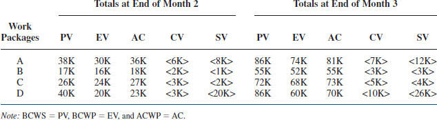
A week after sending the status report to Spokane Industries, Franklin's project manager was asked to attend an emergency meeting requested by Spokane's vice president for engineering, who was functioning as the project sponsor. The vice president was threatening to cancel the project because of poor performance. At the meeting, the vice president commented, “Over the past month the cost variance overrun has increased by 78 percent from $14,000 to $25,000, and the schedule variance slippage has increased by 45 percent from $31,000 to $45,000. At these rates, we are easily looking at a 500 percent cost overrun and a schedule slippage of at least one year. We cannot afford to let this project continue at this lackluster performance rate. If we cannot develop a plan to control time and cost any better than we have in the past three months, then I will just cancel the contract now, and we will find another contractor who can perform.”
QUESTIONS
- Are the vice president's comments about cost and schedule variance correct?
- What information did the vice president fail to analyze?
- What additional information should have been included in the status report?
- Does Franklin Electronics understand earned value measurement? If not, then what went wrong?
- Does Spokane Industries understand project management?
- Does proper earned value measurement serve as a replacement for interchange meetings?
- What should the project manager from Franklin say in his defense?
TROUBLE IN PARADISE
As a reward for becoming Acme Corporation's first PMP, Acme assigned the new PMP, Wiley Coyote, the leadership role of an important project in which the timing of the deliverables was critical to the success of the project. A delay in the schedule could cost Acme a loss of at least $100,000 per month. Wiley Coyote's first responsibility as project manager was the preparation of a solicitation package for the selection of an engineering contractor.
Eight companies prepared bids based on the solicitation package. Wiley Coyote decided to negotiate only with the low bidder, who happened to be at a significantly lower final cost than the other bidders. The contractor's project manager, Ima Roadrunner, would be handling the negotiations for the contractor. This was a contractor that Wiley Coyote had never worked with previously. Wiley Coyote reviewed the critical information in the proposal from the contractor:
- All work would be accomplished by engineering.
- Total burdened labor was 2000 hours at $120/hour.
- The duration of the project would be approximately 6 months and would be completed in 2006 (labor rates might be different in 2007).
- The contractor's overhead rate applied was 150 percent for engineering.
- All of the assigned workers would be at the same pay grade and would be assigned full time for the duration of the project.
- Profit requested was 12.5 percent, but subject to negotiations.
- Ima Roadrunner's salary would be included in the overhead structure.
- No materials were required.
During negotiations, Ima Roadrunner provided Wiley Coyote with the salary structure for engineering, shown in Exhibit 15-1.
Exhibit 15-15. Departmental pay structure
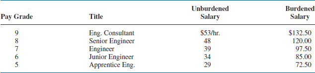
Wiley Coyote asked Ima Roadrunner for the timing (i.e., manpower curve) of when the resources would be assigned. The result, provided by Ima Roadrunner, is shown in Exhibit 15-2 in the format of an S-curve that also shows the payment plan from the customer to the contractor.
The solicitation package identified the contract as a fixed-price contract with penalties for late delivery. Ima Roadrunner argued that the penalty clauses were unfair in their current wording and that a higher profit margin would be required to compensate for the risks. At this point, Wiley Coyote's superior intellect became apparent; he agreed to eliminate the penalty clauses if Ima Roadrunner agreed to lower the profit margin from 12.5 to 10 percent. Ima Roadrunner countered that the contract should then be a fixed-price-incentive-fee contract so that Ima Roadrunner could make up the lost 2.5 percent of profit by completing the project under budget. Both parties agreed to this and the deal was done.
The contract did not call for any type of earned value reporting, but Ima Roadrunner, who had very limited knowledge of earned value measurement and had never used it before, agreed to provide a monthly report that would show simply planned value (BCWS), earned value (BCWP), and actual costs (ACWP). Wiley Coyote agreed to this. After all, now that Wiley Coyote was a PMP, he knew how to extract all of the remaining information, such as variance analyses, cost-at-completion, and cost-to-completion, from these three values in the monthly report.
Exhibit 15-2. S-curve or spending curve
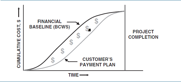
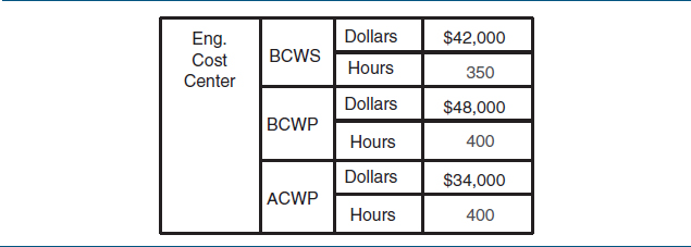
At the end of the first month, Wiley Coyote received the highly simplified earned value status report shown in Exhibit 15-3. Wiley Coyote was delighted with the results thus far. Now it looked like the project would be completed at least one month ahead of schedule and significantly under budget. Wiley Coyote provided Acme with significant cost savings by going with the lowest cost supplier, got the profit margin reduced by 20 percent, and would most likely come in ahead of schedule and at additional cost savings. Wiley Coyote was about to become a “superstar” in the eyes of Acme's executives. Everyone would realize that Wiley Coyote had finally outsmarted the Roadrunner. Wiley Coyote now began planning how he would spend the huge bonus he expected to receive at the completion of the project.
At the end of the fifth month, Ima Roadrunner informed Wiley Coyote of the good news that the project would be completed within cost, but there was also bad news that the completion date would be at the end of month 8, making the project two months late and at a significant loss to Acme Corporation. Wiley Coyote's thoughts on how to spend his bonus were now replaced with creative ideas on how to update his resume. Today, Wiley Coyote is on the lecture circuit discussing ways to identify warning signs of a potential project disaster.
Once again, the Roadrunner outsmarted Wiley Coyote. You have been hired in as a consultant to Acme Corporation to analyze what went wrong and to prepare a list of lessons learned for other project managers. Using the information in the case and all three exhibits, identify what went wrong. Also, were there any early warning signs, especially at the end of the first month, which should have warned Wiley Coyote that disaster might be imminent?
*Case Study also appears at end of chapter.
1. Russell D. Archibald, Managing High-Technology Programs and Projects (New York: John Wiley & Sons, 1976), p. 191.
2. Only three levels of cost reporting are assumed here. If work packages were used, then the WBS number would identify all five levels of control.
3. Russell D. Archibald, Managing High-Technology Programs and Projects (New York: John Wiley & Sons, 1976), p. 176.
4. C. N. Parkinson, Parkinson's Law (Boston: Houghton Mifflin, 1957).
5. These techniques, in addition to the 50/50 method for determining work in progress, are available in software packages.
6. W. Q. Fleming and J. M. Koppelman, “Forecasting the Final Cost and Schedule Results,” PM Network, January 1996, pp. 13-18.
7. Adapted from Quentin W. Fleming, Cost/Schedule Control Systems Criteria (Chicago: Probus Publishers, 1992), pp. 144-145.
8. Adapted from Quentin W. Fleming, Cost/Schedule Control Systems Criteria (Chicago: Probus Publishers, 1992), pp. 151-152.
9. Here we are discussing system specifications. Functional modification responses can also require specification changes, but not on the system level. Examples of functional modifications might be changes in tolerances for testing or for purchasing raw materials.