Pricing and Estimating

14.0 INTRODUCTION

With the complexities involved, it is not surprising that many business managers consider pricing an art. Having information on customer cost budgets and competitive pricing would certainly help. However, the reality is that whatever information is available to one bidder is generally available to the others.

A disciplined approach helps in developing all the input for a rational pricing recommendation. A side benefit of using a disciplined management process is that it leads to the documentation of the many factors and assumptions involved at a later time. These can be compared and analyzed, contributing to the learning experiences that make up the managerial skills needed for effective business decisions.

Estimates are not blind luck. They are well-thought-out decisions based on either the best available information, some type of cost estimating relationship, or some type of cost model. Cost estimating relationships (CERs) are generally the output of cost models. Typical CERs might be:

• Mathematical equations based on regression analysis
• Cost–quantity relationships such as learning curves
• Cost–cost relationships
• Cost–noncost relationships based on physical characteristics, technical parameters, or performance characteristics

14.1 GLOBAL PRICING STRATEGIES

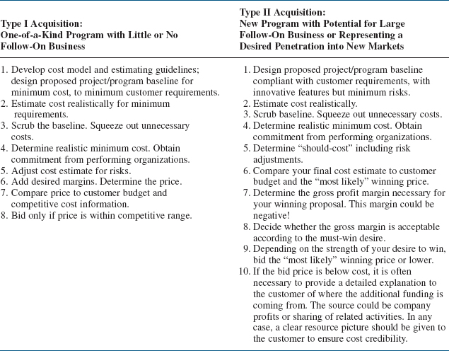
Specific pricing strategies must be developed for each individual situation. Frequently, however, one of two situations prevails when one is pursuing project acquisitions competitively. First, the new business opportunity may be a one-of-a-kind program with little or no follow-on potential, a situation classified as type I acquisition. Second, the new business opportunity may be an entry point to a larger follow-on or repeat business, or may represent a planned penetration into a new market. This acquisition is classified as type II.

Clearly, in each case, we have specific but different business objectives. The objective for type I acquisition is to win the program and execute it profitably and satisfactorily according to contractual agreements. The type II objective is often to win the program and perform well, thereby gaining a foothold in a new market segment or a new customer community in place of making a profit. Accordingly, each acquisition type has its own, unique pricing strategy, as summarized in Table 14-1.

Comparing the two pricing strategies for the two global situations (as shown in Table 14-1) reveals a great deal of similarity for the first five points. The fundamental difference is that for a profitable new business acquisition the bid price is determined according to actual cost, whereas in a “must-win” situation the price is determined by the market forces. It should be emphasized that one of the most crucial inputs in the pricing decision is the cost estimate of the proposed baseline. The design of this baseline to the minimum requirements should be started early, in accordance with well-defined ground rules, cost models, and established cost targets. Too often the baseline design is performed in parallel with the proposal development. At the proposal stage it is too late to review and fine-tune the baseline for minimum cost. Also, such a late start does not allow much of an option for a final bid decision. Even if the price appears outside the competitive range, it makes little sense to terminate the proposal development. As all the resources have been sent anyway, one might just as well submit a bid in spite of the remote chance of winning.

Clearly, effective pricing begins a long time before proposal development. It starts with preliminary customer requirements, well-understood subtasks, and a top-down estimate with should-cost targets. This allows the functional organization to design a baseline to meet the customer requirements and cost targets, and gives management the time to review and redirect the design before the proposal is submitted. Furthermore, it gives management an early opportunity to assess the chances of winning during the acquisition cycle, at a point when additional resources can be allocated or the acquisition effort can be terminated before too many resources are committed to a hopeless effort.

TABLE 14-1. TWO GLOBAL PRICING STRATEGIES

The final pricing review session should be an integration and review of information already well known in its basic context. The process and management tools outlined here should help to provide the framework and discipline for deriving pricing decisions in an orderly and effective way.

14.2 TYPES OF ESTIMATES

Any company or corporation that wants to remain profitable must continuously improve its estimating and pricing methodologies. While it is true that some companies have been successful without good cost estimating and pricing, very few remain successful without them.

Good estimating requires that information be collected prior to the initiation of the estimating process. Typical information includes:

• Recent experience in similar work
• Professional and reference material
• Market and industry surveys
• Knowledge of the operations and processes
• Estimating software and databases if available
• Interviews with subject matter experts

Projects can range from a feasibility study, through modification of existing facilities, to complete design, procurement, and construction of a large complex. Whatever the project may be, whether large or small, the estimate and type of information desired may differ radically.

The first type of estimate is an order-of-magnitude analysis, which is made without any detailed engineering data. The order-of-magnitude analysis may have an accuracy of ±35 percent within the scope of the project. This type of estimate may use past experience (not necessarily similar), scale factors, parametric curves, or capacity estimates (i.e., $/# of product or $/kW electricity).

Order-of-magnitude estimates are top-down estimates usually applied to level 1 of the WBS, and in some industries, use of parametric estimates are included. A parametric estimate is based upon statistical data. For example, assume that you live in a Chicago suburb and wish to build the home of your dreams. You contact a construction contractor who informs you that the parametric or statistical cost for a home in this suburb is $120 per square foot. In Los Angeles, the cost may be $4150 per square foot.

Next, there is the approximate estimate (or top-down estimate), which is also made without detailed engineering data, and may be accurate to ± 15 percent. This type of estimate is prorated from previous projects that are similar in scope and capacity, and may be titled as estimating by analogy, parametric curves, rule of thumb, and indexed cost of similar activities adjusted for capacity and technology. In such a case, the estimator may say that this activity is 50 percent more difficult than a previous (i.e., reference) activity and requires 50 percent more time, man-hours, dollars, materials, and so on.

The definitive estimate, or grassroots buildup estimate, is prepared from well-defined engineering data including (as a minimum) vendor quotes, fairly complete plans, specifications, unit prices, and estimate to complete. The definitive estimate, also referred to as detailed estimating, has an accuracy of ± 5 percent.

Another method for estimating is the use of learning curves. Learning curves are graphical representations of repetitive functions in which continuous operations will lead to a reduction in time, resources, and money. The theory behind learning curves is usually applied to manufacturing operations.

Each company may have a unique approach to estimating. However, for normal project management practices, Table 14-2 would suffice as a starting point.

Many companies try to standardize their estimating procedures by developing an estimating manual. The estimating manual is then used to price out the effort, perhaps as much as 90 percent. Estimating manuals usually give better estimates than industrial engineering standards because they include groups of tasks and take into consideration such items as downtime, cleanup time, lunch, and breaks. Table 14-3 shows the table of contents for a construction estimating manual.

TABLE 14-2. STANDARD PROJECT ESTIMATING

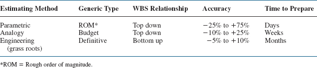
TABLE 14-3. ESTIMATING MANUAL TABLE OF CONTENTS

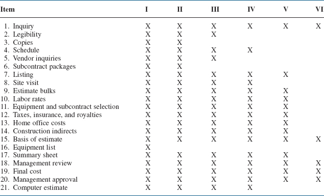
Estimating manuals, as the name implies, provide estimates. The question, of course, is “How good are the estimates?” Most estimating manuals provide accuracy limitations by defining the type of estimates (shown in Table 14-3). Using Table 14-3, we can create Tables 14-4, 14-5, and 14-6, which illustrate the use of the estimating manual.

Not all companies can use estimating manuals. Estimating manuals work best for repetitive tasks or similar tasks that can use a previous estimate adjusted by a degree-of-difficulty factor. Activities such as R&D do not lend themselves to the use of estimating manuals other than for benchmark, repetitive laboratory tests. Proposal managers must carefully consider whether the estimating manual is a viable approach. The literature abounds with examples of companies that have spent millions trying to develop estimating manuals for situations that just do not lend themselves to the approach.

TABLE 14-4. CLASSES OF ESTIMATES

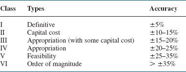
TABLE 14-5. CHECKLIST FOR WORK NORMALLY REQUIRED FOR THE VARIOUS CLASSES (I-VI) OF ESTIMATES

During competitive bidding, it is important that the type of estimate be consistent with the customer's requirements. For in-house projects, the type of estimate can vary over the life cycle of a project:

• Conceptual stage: Venture guidance or feasibility studies for the evaluation of future work. This estimating is often based on minimum-scope information.
• Planning stage: Estimating for authorization of partial or full funds. These estimates are based on preliminary design and scope.
• Main stage: Estimating for detailed work.
• Termination stage: Reestimation for major scope changes or variances beyond the authorization range.

14.3 PRICING PROCESS

This activity schedules the development of the work breakdown structure and provides management with two of the three operational tools necessary for the control of a system or project. The development of these two tools is normally the responsibility of the program office with input from the functional units.

The integration of the functional unit into the project environment or system occurs through the pricing-out of the work breakdown structure. The total program costs obtained by pricing out the activities over the scheduled period of performance provide management with the third tool necessary to successfully manage the project. During the pricing activities, the functional units have the option of consulting program management about possible changes in the activity schedules and work breakdown structure.

TABLE 14-6. DATA REQUIRED FOR PREPARATION OF ESTIMATES

The work breakdown structure and activity schedules are priced out through the lowest pricing units of the company. It is the responsibility of these pricing units, whether they be sections, departments, or divisions, to provide accurate and meaningful cost data (based on historical standards, if possible). All information is priced out at the lowest level of performance required, which, from the assumption of Chapter 11, will be the task level. Costing information is rolled up to the project level and then one step further to the total program level.

Under ideal conditions, the work required (i.e., man-hours) to complete a given task can be based on historical standards. Unfortunately, for many industries, projects and programs are so diversified that realistic comparison between previous activities may not be possible. The costing information obtained from each pricing unit, whether or not it is based on historical standards, should be regarded only as an estimate. How can a company predict the salary structure three years from now? What will be the cost of raw materials two years from now? Will the business base (and therefore overhead rates) change over the duration of the program? The final response to these questions shows that costing data are explicitly related to an environment that cannot be predicted with any high degree of certainty. The systems approach to management, however, provides for a more rapid response to the environment than less structured approaches permit.

Once the cost data are assembled, they must be analyzed for their potential impact on the company resources of people, money, equipment, and facilities. It is only through a total program cost analysis that resource allocations can be analyzed. The resource allocation analysis is performed at all levels of management, ranging from the section supervisor to the vice president and general manager. For most programs, the chief executive must approve final cost data and the allocation of resources.

Proper analysis of the total program costs can provide management (both program and corporate) with a strategic planning model for integration of the current program with other programs in order to obtain a total corporate strategy. Meaningful planning and pricing models include analyses for monthly manloading schedules per department, monthly costs per department, monthly and yearly total program costs, monthly material expenditures, and total program cash-flow and man-hour requirements per month.

Previously we identified several of the problems that occur at the nodes where the horizontal hierarchy of program management interfaces with the vertical hierarchy of functional management. The pricing-out of the work breakdown structure provides the basis for effective and open communication between functional and program management where both parties have one common goal. This is shown in Figure 14-1. After the pricing effort is completed, and the program is initiated, the work breakdown structure still forms the basis of a communications tool by documenting the performance agreed on in the pricing effort, as well as establishing the criteria against which performance costs will be measured.

14.4 ORGANIZATIONAL INPUT REQUIREMENTS

Once the work breakdown structure and activity schedules are established, the program manager calls a meeting for all organizations that will submit pricing information. It is imperative that all pricing or labor-costing representatives be present for the first meeting. During this “kickoff” meeting, the work breakdown structure is described in depth so that each pricing unit manager will know exactly what his responsibilities are during the program. The kickoff meeting also resolves the struggle for power among functional managers whose responsibilities may be similar. An example of this would be quality control activities. During the research and development phase of a program, research personnel may be permitted to perform their own quality control efforts, whereas during production activities the quality control department or division would have overall responsibility. Unfortunately, one meeting is not always sufficient to clarify all problems. Follow-up or status meetings are held, normally with only those parties concerned with the problems that have arisen. Some companies prefer to have all members attend the status meetings so that all personnel will be familiar with the total effort and the associated problems. The advantage of not having all program-related personnel attend is that time is of the essence when pricing out activities. Many functional divisions carry this policy one step further by having a divisional representative together with possibly key department managers or section supervisors as the only attendees at the kickoff meeting. The divisional representative then assumes all responsibility for assuring that all costing data are submitted on time. This arrangement may be beneficial in that the program office need contact only one individual in the division to learn of the activity status, but it may become a bottleneck if the representative fails to maintain proper communication between the functional units and the program office, or if the individual simply is unfamiliar with the pricing requirements of the work breakdown structure.

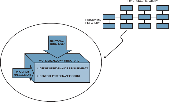
FIGURE 14-1. The vertical-horizontal interface.

During proposal activities, time may be extremely important. There are many situations in which a request for proposal (RFP) requires that all responders submit their bids by a specific date. Under a proposal environment, the activities of the program office, as well as those of the functional units, are under a schedule set forth by the proposal manager. The proposal manager's schedule has very little, if any, flexibility and is normally under tight time constraints so that the proposal may be typed, edited, and published prior to the date of submittal. In this case, the RFP will indirectly define how much time the pricing units have to identify and justify labor costs.

The justification of the labor costs may take longer than the original cost estimates, especially if historical standards are not available. Many proposals often require that comprehensive labor justification be submitted. Other proposals, especially those that request an almost immediate response, may permit vendors to submit labor justification at a later date.

In the final analysis, it is the responsibility of the lowest pricing unit supervisors to maintain adequate standards, so that an almost immediate response can be given to a pricing request from a program office.

14.5 LABOR DISTRIBUTIONS

The functional units supply their input to the program office in the form of man-hours, as shown in Figure 14-2. The input may be accompanied by labor justification, if required. The man-hours are submitted for each task, assuming that the task is the lowest pricing element, and are time-phased per month. The man-hours per month per task are converted to dollars after multiplication by the appropriate labor rates. The labor rates are generally known with certainty over a twelve-month period, but from then on are only estimates. How can a company predict salary structures five years hence? If the company underestimates the salary structure, increased costs and decreased profits will occur. If the salary structure is overestimated, the company may not be competitive; if the project is government funded, then the salary structure becomes an item under contract negotiations.

The development of the labor rates to be used in the projection is based on historical costs in business base hours and dollars for the most recent month or quarter. Average hourly rates are determined for each labor unit by direct effort within the operations at the department level. The rates are only averages, and include both the highest-paid employees and lowest-paid employees, together with the department manager and the clerical support.¹ These base rates are then escalated as a percentage factor based on past experience, budget as approved by management, and the local outlook and similar industries. If the company has a predominant aerospace or defense industry business base, then these salaries are negotiated with local government agencies prior to submittal for proposals.

The labor hours submitted by the functional units are quite often overestimated for fear that management will “massage” and reduce the labor hours while attempting to maintain the same scope of effort. Many times management is forced to reduce man-hours either because of insufficient funding or just to remain competitive in the environment. The reduction of man-hours often causes heated discussions between the functional and program managers. Program managers tend to think in terms of the best interests of the program, whereas functional managers lean toward maintaining their present staff.

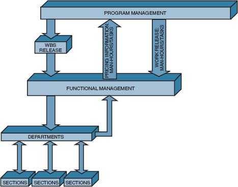
FIGURE 14-2. Functional pricing flow.

The most common solution to this conflict rests with the program manager. If the program manager selects members for the program team who are knowledgeable in man-hour standards for each of the departments, then an atmosphere of trust can develop between the program office and the functional department so that man-hours can be reduced in a manner that represents the best interests of the company. This is one of the reasons why program team members are often promoted from within the functional ranks.

The man-hours submitted by the functional units provide the basis for total program cost analysis and program cost control. To illustrate this process, consider Example 14-1 below.

Example 14-1. On May 15, Apex Manufacturing decided to enter into competitive bidding for the modification and updating of an assembly line program. A work breakdown structure was developed as shown below:

On June 1, each pricing unit was given the work breakdown structure together with the schedule shown in Figure 14-3. According to the schedule developed by the proposal manager for this project, all labor data must be submitted to the program office for review no later than June 15. It should be noted here that, in many companies, labor hours are submitted directly to the pricing department for submittal into the base case computer run. In this case, the program office would “massage” the labor hours only after the base case figures are available. This procedure assumes that sufficient time exists for analysis and modification of the base case. If the program office has sufficient personnel capable of critiquing the labor input prior to submittal to the base case, then valuable time can be saved, especially if two or three days are required to obtain computer output for the base case.

During proposal activities, the proposal manager, pricing manager, and program manager must all work together, although the program manager has the final say. The primary responsibility of the proposal manager is to integrate the proposal activities into the operational system so that the proposal will be submitted to the requestor on time. A typical schedule developed by the proposal manager is shown in Figure 14-4. The schedule includes all activities necessary to “get the proposal out of the house,” with the first major step being the submittal of man-hours by the pricing organizations. Figure 14-4 also indicates the tracking of proposal costs. The proposal activity schedule is usually accompanied by a time schedule with a detailed estimates checklist if the complexity of the proposal warrants one. The checklist generally provides detailed explanations for the proposal activity schedule.

After the planning and pricing charts are approved by program team members and program managers, they are entered into an electronic data processing (EDP) system as shown in Figure 14-5. The computer then prices the hours on the planning charts using the applicable department rates for preparation of the direct budget time plan and estimate-at-completion reports. The direct budget time plan reports, once established, remain the same for the life of the contract except for customer-directed or approved changes or when contractor management determines that a reduction in budget is advisable. However, if a budget is reduced by management, it cannot be increased without customer approval.

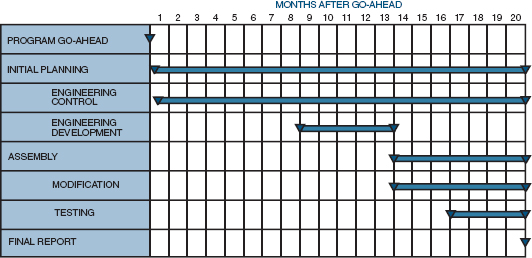
FIGURE 14-3. Activity schedule for assembly line updating.

FIGURE 14-4. Proposal activity schedule.

The time plan is normally a monthly mechanical printout of all planned effort by work package and organizational element over the life of the contract, and serves as the data bank for preparing the status completion reports.

Initially, the estimate-at-completion report is identical to the budget report, but it changes throughout the life of a program to reflect degradation or improvement in performance or any other events that will change the program cost or schedule.

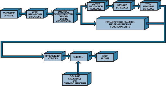
FIGURE 14-5. Labor planning flowchart.

14.6 OVERHEAD RATES

The ability to control program costs involves more than tracking labor dollars and labor hours; overhead dollars, one of the biggest headaches, must also be tracked. Although most programs have an assistant program manager for cost whose responsibilities include monthly overhead rate analysis, the program manager can drastically increase the success of his program by insisting that each program team member understand overhead rates. For example, if overhead rates apply only to the first forty hours of work, then, depending on the overhead rate, program dollars can be saved by performing work on overtime where the increased salary is at a lower burden. This can be seen in Example 14–2 below.

Example 14–2. Assume that ApexManufacturing must write an interim report for task 1 of project 1 during regular shift or on overtime. The project will require 500 man-hours at $15.00 per hour. The overhead burden is 75 percent on regular shift but only 5 percent on overtime. Overtime, however, is paid at a rate of time and a half. Assuming that the report can be written on either time, which is cost-effective—regular time or overtime?

• On regular time the total cost is:

  (500 hours) × ($15.00/hour) × (100% + 75% burden) = $13,125.00

• On overtime, the total cost is:

  (500 hours) × ($15.00/hour × 1.5 overtime) × (100% + 5% burden) = $11,812.50

Therefore, the company can save $1,312.50 by performing the work on overtime. Scheduling overtime can produce increased profits if the overtime overhead rate burden is much less than the regular time burden. This difference can be very large in manufacturing divisions, where overhead rates between 300 and 450 percent are common.

Regardless of whether one analyzes a project or a system, all costs must have associated overhead rates. Unfortunately, many program managers and systems managers consider overhead rates as a magic number pulled out of the air. The preparation and assignment of overheads to each of the functional divisions is a science. Although the total dollar pool for overhead rates is relatively constant, management retains the option of deciding how to distribute the overhead among the functional divisions. A company that supports its R&D staff through competitive bidding projects may wish to keep the R&D overhead rate as low as possible. Care must be taken, however, that other divisions do not absorb additional costs so that the company no longer remains competitive on those manufactured products that may be its bread and butter.

The development of the overhead rates is a function of three separate elements: direct labor rates, direct business base projections, and projection of overhead expenses. Direct labor rates have already been discussed. The direct business base projection involves the determination of the anticipated direct labor hours and dollars along with the necessary direct materials and other direct costs required to perform and complete the program efforts included in the business base. Those items utilized in the business base projection include all contracted programs as well as the proposed or anticipated efforts. The foundation for determination of the business base required for each program can be one or more of the following:

• Actual costs to date and estimates to completion
• Proposal data
• Marketing intelligence
• Management goals
• Past performance and trends

The projection of the overhead expenses is made by an analysis of each of the elements that constitute the overhead expense. A partial listing of those items is shown in Table 14-7. Projection of expenses within the individual elements is then made based on one or more of the following:

• Historical direct/indirect labor ratios
• Regression and correlation analysis
• Manpower requirements and turnover rates
• Changes in public laws
• Anticipated changes in company benefits
• Fixed costs in relation to capital asset requirements
• Changes in business base
• Bid and proposal (B&P) tri-service agreements
• Internal research and development (IR&D) tri-service agreements

For many industries, such as aerospace and defense, the federal government funds a large percentage of the B&P and IR&D activities. This federal funding is a necessity since many companies could not otherwise be competitive within the industry. The federal government employs this technique to stimulate research and competition. Therefore, B&P and IR&D are included in the above list.

TABLE 14-7. ELEMENTS OF OVERHEAD RATES

The prime factor in the control of overhead costs is the annual budget. This budget, which is the result of goals and objectives established by the chief executive officer, is reviewed and approved at all levels of management. it is established at department level, and the department manager has direct responsibility for identifying and controlling costs against the approved plan.

The departmental budgets are summarized, in detail, for higher levels of management. This summarization permits management, at these higher organizational levels, to be aware of the authorized indirect budget in their area of responsibility.

Reports are published monthly indicating current month and year-to-date budget, actuals, and variances. These reports are published for each level of management, and an analysis is made by the budget department through coordination and review with management. Each directorate's total organization is then reviewed with the budget analyst who is assigned the overhead cost responsibility. A joint meeting is held with the directors and the vice president and general manager, at which time overhead performance is reviewed.

14.7 MATERIALS/SUPPORT COSTS

The salary structure, overhead structure, and labor hours fulfill three of four major pricing input requirements. The fourth major input is the cost for materials and support. Six subtopics are included under materials/support: materials, purchased parts, subcontracts, freight, travel, and other. Freight and travel can be handled in one of two ways, both normally dependent on the size of the program. For small-dollar-volume programs, estimates are made for travel and freight. For large-dollar-volume programs, travel is normally expressed as between 3 and 5 percent of the direct labor costs, and freight is likewise between 3 and 5 percent of all costs for material, purchased parts, and subcontracts. The category labeled “other support costs” may include such topics as computer hours or specialconsultants.

FIGURE 14-6. Material planning flowchart.

Determination of the material costs is very time-consuming, more so than cost determination for labor hours. Material costs are submitted via a bill of materials that includes all vendors from whom purchases will be made, projected costs throughout the program, scrap factors, and shelf lifetime for those products that may be perishable.

Upon release of the work statement, work breakdown structure, and subdivided work description, the end-item bill of materials and manufacturing plans are prepared as shown in Figure 14-6. End-item materials are those items identified as an integral part of the production end-item. Support materials consist of those materials required by engineering and operations to support the manufacture of end-items, and are identified on the manufacturing plan.

A procurement plan/purchase requisition is prepared as soon as possible after contract negotiations (using a methodology as shown in Figure 14-7). This plan is used to monitor material acquisitions, forecast inventory levels, and identify material price variances.

Manufacturing plans prepared upon release of the subdivided work descriptions are used to prepare tool lists for manufacturing, quality assurance, and engineering. From these plans a special tooling breakdown is prepared by tool engineering, which defines those tools to be procured and the material requirements of tools to be fabricated in-house. These items are priced by cost element for input on the planning charts.

The materials/support costs are submitted by month for each month of the program. If long-lead funding of materials is anticipated, then they should be assigned to the first month of the program. In addition, an escalation factor for costs of materials/support items must be applied to all materials/support costs. Some vendors may provide fixed prices over time periods in excess of a twelve-month period. As an example, vendor Z may quote a firm-fixed price of $130.50 per unit for 650 units to be delivered over the next eighteen months if the order is placed within sixty days. There are additional factors that influence the cost of materials.

FIGURE 14-7. Procurement activity.

14.8 PRICING OUT THE WORK

Using logical pricing techniques will help in obtaining detailed estimates. The following thirteen steps provide a logical sequence to help a company control its limited resources. These steps may vary from company to company.

Although the pricing of a project is an iterative process, the project manager must still develop cost summary reports at each iteration point so that key project decisions can be made during the planning. Detailed pricing summaries are needed at least twice: in preparation for the pricing review meeting with management and at pricing termination. At all other times it is possible that “simple cosmetic surgery” can be performed on previous cost summaries, such as perturbations in escalation factors and procurement cost of raw materials. The list below shows the typical pricing reports:

• A detailed cost breakdown for each WBS element. If the work is priced out at the task level, then there should be a cost summary sheet for each task, as well as rollup sheets for each project and the total program.
• A total program manpower curve for each department. These manpower curves show how each department has contracted with the project office to supply functional resources. If the departmental manpower curves contain several “peaks and valleys,” then the project manager may have to alter some of his schedules to obtain some degree of manpower smoothing. Functional managers always prefer manpower-smoothed resource allocations.
• A monthly equivalent manpower cost summary. This table normally shows the fully burdened cost for the average departmental employee carried out over the entire period of project performance. If project costs have to be reduced, the project manager performs a parametric study between this table and the manpower curve tables.
• A yearly cost distribution table. This table is broken down by WBS element and shows the yearly (or quarterly) costs that will be required. This table, in essence, is a project cash-flow summary per activity.
• A functional cost and hour summary. This table provides top management with an overall description of how many hours and dollars will be spent by each major functional unit, such as a division. Top management would use this as part of the forward planning process to make sure that there are sufficient resources available for all projects. This also includes indirect hours and dollars.
• A monthly labor hour and dollar expenditure forecast. This table can be combined with the yearly cost distribution, except that it is broken down by month, not activity or department. In addition, this table normally includes manpower termination liability information for premature cancellation of the project by outside customers.
• A raw material and expenditure forecast. This shows the cash flow for raw materials based on vendor lead times, payment schedules, commitments, and termination liability.
• Total program termination liability per month. This table shows the customer the monthly costs for the entire program. This is the customer's cash flow, not the contractor's. The difference is that each monthly cost contains the termination liability for man-hours and dollars, on labor and raw materials. This table is actually the monthly costs attributed to premature project termination.

These tables are used by project managers as the basis for project cost control and by upper-level executives for selecting, approving, and prioritizing projects.

14.9 SMOOTHING OUT DEPARTMENT MAN-HOURS

The dotted curve in Figure 14-8 indicates projected manpower requirements for a given department as a result of a typical program manloading schedule. Department managers, however, attempt to smooth out the manpower curve as shown by the solid line in Figure 14-8. Smoothing out the manpower requirements benefits department managers by eliminating fractional man-hours per day. The program manager must understand that if departments are permitted to eliminate peaks, valleys, and small-step functions in manpower planning, small project and task man-hour (and cost) variances can occur, but should not, in general, affect the total program cost significantly.

Two important questions to ask are whether the department has sufficient personnel available to fulfill manpower requirements and what is the rate at which the functional departments can staff the program? For example, project engineering requires approximately twenty-three people during January 2002. The functional manager, however, may have only fifteen people available for immediate reassignment, with the remainder to be either transferred from other programs or hired from outside the company. The same situation occurs during activity termination. Will project engineering still require twenty-three people in August 2002, or can some of these people begin being phased to other programs, say, as early as June 2002? This question, specifically addressed to support and administrative tasks/projects, must be answered prior to contract negotiations. Figure 14-9 indicates the types of problems that can occur. Curve A shows the manpower requirements for a given department after time-smoothing. Curve B represents the modification to the time-phase curve to account for reasonable program manning and demanning rates. The difference between these two curves (i.e., the shaded area) therefore reflects the amount of money the contractor may have to forfeit owing to manning and demanning activities. This problem can be partially overcome by increasing the manpower levels after time-smoothing (see curve C) such that the difference between curves B and C equals the amount of money that would be forfeited from curves A and B. Of course, program management would have to be able to justify this increase in average manpower requirements, especially if the adjustments are made in a period of higher salaries and overhead rates.

FIGURE 14-8. Typical manpower loading.

FIGURE 14-9. Linearly increased manpower loading.

14.10 THE PRICING REVIEW PROCEDURE

The ability to project, analyze, and control problem costs requires coordination of pricing information and cooperation between the functional units and upper-level management. A typical company policy for cost analysis and review is shown in Figure 14-10. Corporate management may be required to initiate or authorize activities, if corporate/company resources are or may be strained by the program, if capital expenditures are required for new facilities or equipment, or simply if corporate approval is required for all projects in excess of a certain dollar amount.

Upper-level management, upon approval by the chief executive officer of the company, approves and authorizes the initiation of the project or program. The actual performance activities, however, do not begin until the director of program management selects a program manager and authorizes either the bid and proposal budget (if the program is competitive) or project planning funds.

The newly appointed program manager then selects this program's team. Team members, who are also members of the program office, may come from other programs, in which case the program manager may have to negotiate with other program managers and upper-level management to obtain these individuals. The members of the program office are normally support-type individuals. In order to obtain team members representing the functional departments, the program manager must negotiate directly with the functional managers. Functional team members may not be selected or assigned to the program until the actual work is contracted for. Many proposals, however, require that all functional team members be identified, in which case selection must be made during the proposal stage of a program.

The first responsibility of the program office (not necessarily including functional team members) is the development of the activity schedules and the work breakdown structure. The program office then provides work authorization for the functional units to price out the activities. The functional units then submit the labor hours, material costs, and justification, if required, to the pricing team member. The pricing team member is normally attached to the program office until the final costs are established, and becomes part of the negotiating team if the project is competitive.

Once the base case is formulated, the pricing team member, together with the other program office team members, performs perturbation analyses. These analyses are designed as systems approaches to problem-solving where alternatives are developed in order to respond to management's questions during the final review.

FIGURE 14-10. The pricing review procedure.

The base case, with the perturbation analysis costs, is then reviewed with upper-level management in order to formulate a company position for the program and to take a hard look at the allocation of resources required for the program. The company position may be to cut costs, authorize work, or submit a bid. Corporate approval may be required if the company's chief executive officer has a ceiling on the amount he can authorize.

If labor costs must be cut, the program manager must negotiate with the functional managers as to the size and method for the cost reductions. Otherwise, this step would simply entail authorization for the functional managers to begin the activities.

Figure 14-10 represents the system approach to determining total program costs. This procedure normally creates a synergistic environment, provides open channels of communication between all levels of management, and ensures agreement among all individuals as to program costs.

14.11 SYSTEMS PRICING

The systems approach to pricing out the activity schedules and the work breakdown structure provide a means for obtaining unity within the company. The flow of information readily admits the participation of all members of the organization in the program, even if on a part-time basis. Functional managers obtain a better understanding of how their labor fits into the total program and how their activities interface with those of other departments. For the first time, functional managers can accurately foresee how their activity can lead to corporate profits.

FIGURE 14-11. System approach to resource control.

The project pricing model (sometimes called a strategic project planning model) acts as a management information system, forming the basis for the systems approach to resource control, as shown in Figure 14-11. The summary sheets from the computer output of the strategic pricing model help management select programs that will best utilize resources. The strategic pricing model also provides management with an invaluable tool for performing perturbation analysis on the base case costs and an opportunity for design and evaluation of contingency plans, if necessary.

14.12 DEVELOPING THE SUPPORTING/BACKUP COSTS

Not all cost proposals require backup support, but for those that do, the backup support should be developed along with the pricing. The itemized prices should be compatible with the supporting data. Government pricing requirements are a special case.

Most supporting data come from external (subcontractor or outside vendor) quotes. Internal data must be based on historical data, and these historical data must be updated continually as each new project is completed. The supporting data should be traceable by itemized charge numbers.

Customers may wish to audit the cost proposal. In this case, the starting point might be the supporting data. It is not uncommon on sole-source proposals to have the supporting data audited before the final cost proposal is submitted to the customer.

Not all cost proposals require supporting data; the determining factor is usually the type of contract. On a fixed-price effort, the customer may not have the right to audit your books. However, for a cost-reimbursable package, your costs are an open book, and the customer usually compares your exact costs to those of the backup support.

Most companies usually have a choice of more than one estimate to be used for backup support. In deciding which estimate to use, consideration must be given to the possibility of follow-on work:

• If your actual costs grossly exceed your backup support estimates, you may lose credibility for follow-on work.
• If your actual costs are less than the backup costs, you must use the new actual costs on follow-on efforts.

The moral here is that backup support costs provide future credibility. If you have well-documented, “livable” cost estimates, then you may wish to include them in the cost proposal even if they are not required.

Since both direct and indirect costs may be negotiated separately as part of a contract, supporting data, such as those in Tables 14-8 through 14-11 and Figure 14-12, may be necessary to justify any costs that may differ from company (or customer-approved) standards.

TABLE 14-8. OPERATIONS SKILLS MATRIX

TABLE 14-9. CONTRACTOR'S MANPOWER AVAILABILITY

TABLE 14-10. STAFF TURNOVER DATA

TABLE 14-11. STAFF EXPERIENCE PROFILE

FIGURE 14-12. Total reimbursable manpower.

14.13 THE LOW-BIDDER DILEMMA

There is little argument about the importance of the price tag to the proposal. The question is, what price will win the job? The decision process that leads to the final price of your proposal is highly complex with many uncertainties. Yet proposal managers, driven by the desire to win the job, may think that a very low-priced proposal will help. But winning is only the beginning. Companies have short- and long-range objectives on profit, market penetration, new product development, and so on. These objectives may be incompatible with or irrelevant to a low-price strategy. For example:

• A suspiciously low price, particularly on cost-plus type proposals, might be perceived by the customer as unrealistic, thus affecting the bidder's cost credibility or even the technical ability to perform.
• The bid price may be unnecessarily low, relative to the competition and customer budget, thus eroding profits.
• The price may be irrelevant to the bid objective, such as entering a new market. Therefore, the contractor has to sell the proposal in a credible way, e.g., using cost sharing.
• Low pricing without market information is meaningless. The price level is always relative to (1) the competitive prices, (2) the customer budget, and (3) the bidder's cost estimate.
• The bid proposal and its price may cover only part of the total program. The ability to win phase II or follow-on business depends on phase I performance and phase II price.
• The financial objectives of the customer may be more complex than just finding the lowest bidder. They may include cost objectives for total system life-cycle cost (LCC), for design to unit production cost (DTUPC), or for specific logistic support items. Presenting sound approaches for attaining these system cost-performance parameters and targets may be just as important as, if not more important than, a low bid for the system's development.

Further, it is refreshing to note that in spite of customer pressures toward low cost and fixed price, the lowest bidder is certainly not an automatic winner. Both commercial and governmental customers are increasingly concerned about cost realism and the ability to perform under contract. A compliant, sound, technical and management proposal, based on past experience with realistic, well-documented cost figures, is often chosen over the lowest bidder, who may project a risky image regarding technical performance, cost, or schedule.

14.14 SPECIAL PROBLEMS

There are always special problems that, if overlooked, can have a severe impact on the pricing effort. As an example, pricing must include an understanding of cost control—specifically, how costs are billed back to the project. There are three possible situations:

• Work is priced out at the department average, and all work performed is charged to the project at the department average salary, regardless of who accomplished the work. This technique is obviously the easiest, but encourages project managers to fight for the highest salary resources, since only average wages are billed to the project.
• Work is priced out at the department average, but all work performed is billed back to the project at the actual salary of those employees who perform the work. This method can create a severe headache for the project manager if he tries to use only the best employees on his project. If these employees are earning substantially more money than the department average, then a cost overrun will occur unless the employees can perform the work in less time. Some companies are forced to use this method by government agencies and have estimating problems when the project that has to be priced out is of a short duration where only the higher-salaried employees can be used. In such a situation it is common to “inflate” the direct labor hours to compensate for the added costs.
• The work is priced out at the actual salary of those employees who will perform the work, and the cost is billed back the same way. This method is the ideal situation as long as the people can be identified during the pricing effort.

Some companies use a combination of all three methods. In this case, the project office is priced out using the third method (because these people are identified early), whereas the functional employees are priced out using the first or second method.

14.15 ESTIMATING PITFALLS

Several pitfalls can impede the pricing function. Probably the most serious pitfall, and the one that is usually beyond the control of the project manager, is the “buy-in” decision, which is based on the assumption that there will be “bail-out” changes or follow-on contracts later. These changes and/or contracts may be for spare parts, maintenance, maintenance manuals, equipment surveillance, optional equipment, optional services, and scrap factors. Other types of estimating pitfalls include:

• Misinterpretation of the statement of work
• Omissions or improperly defined scope
• Poorly defined or overly optimistic schedule
• Inaccurate work breakdown structure
• Applying improper skill levels to tasks
• Failure to account for risks
• Failure to understand or account for cost escalation and inflation
• Failure to use the correct estimating technique
• Failure to use forward pricing rates for overhead, general and administrative, and indirect costs

Unfortunately, many of these pitfalls do not become evident until detected by the cost control system, well into the project.

14.16 ESTIMATING HIGH-RISK PROJECTS

Whether a project is high-risk or low-risk depends on the validity of the historical estimate. Construction companies have well-defined historical standards, which lowers their risk, whereas many R&D and MIS projects are high risk. Typical accuracies for each level of the WBS are shown in Table 14-12.

A common technique used to estimate high-risk projects is the “rolling wave” or “moving window” approach. This is shown in Figure 14-13 for a high-risk R&D project. The project lasts for twelve months. The R&D effort to be accomplished for the first six months is well defined and can be estimated to level 5 of the WBS. However, the effort for the latter six months is based on the results of the first six months and can be estimated at level 2 only, thus incurring a high risk. Now consider part B of Figure 14-13, which shows a six-month moving window. At the end of the first month, in order to maintain a six-month moving window (at level 5 of the WBS), the estimate for month seven must be improved from a level-2 to a level-5 estimate. Likewise, in parts C and D of Figure 14-13, we see the effects of completing the second and third months.

There are two key points to be considered in utilizing this technique. First, the length of the moving window can vary from project to project, and usually increases in length as you approach downstream life-cycle phases. Second, this technique works best when upper-level management understands how the technique works. All too often senior management hears only one budget and schedule number during project approval and might not realize that at least half of the project might be time/cost accurate to only 50-60 percent. Simply stated, when using this technique, the word “rough” is not synonymous with the word “detailed.”

Methodologies can be developed for assessing risk. Figures 14-14, 14-15, and Table 14-13 show such methodologies.

TABLE 14-12. LOW- VERSUS HIGH-RISK ACCURACIES

FIGURE 14-13. The moving window/rolling wave concept.

14.17 PROJECT RISKS

Project plans are “living documents” and are therefore subject to change. Changes are needed in order to prevent or rectify unfortunate situations. These unfortunate situations can be called project risks.

Risk refers to those dangerous activities or factors that, if they occur, will increase the probability that the project's goals of time, cost, and performance will not be met. Many risks can be anticipated and controlled. Furthermore, risk management must be an integral part of project management throughout the entire life cycle of the project.

Some common risks include:

• Poorly defined requirements
• Lack of qualified resources
• Lack of management support
• Poor estimating
• Inexperienced project manager

Risk identification is an art. It requires the project manager to probe, penetrate, and analyze all data. Tools that can be used by the project manager include:

• Decision support systems
• Expected value measures
• Trend analysis/projections
• Independent reviews and audits

FIGURE 14-14. Decision elements for risk contingencies.

FIGURE 14-15. Elements of base cost and risk contingencies.

Managing project risks is not as difficult as it may seem. There are six steps in the risk management process:

• Identification of the risk
• Quantifying the risk
• Prioritizing the risk
• Developing a strategy for managing the risk

TABLE 14-13. STANDARD FORM FOR PROJECT RISK ANALYSIS AND RISK CONTINGENCIES

• Project sponsor/executive review
• Taking action

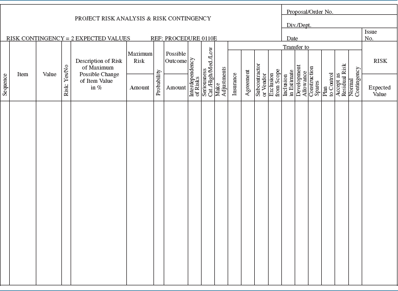
Figures 14-14 and 14-15 and Table 14-13 identify the process of risk evaluation on capital projects. In all three exhibits, it is easily seen that the attempt is to quantify the risks, possibly by developing a contingency fund.

14.18 THE DISASTER OF APPLYING THE 10 PERCENT SOLUTION TO PROJECT ESTIMATES

Economic crunches can and do create chaos in all organizations. For the project manager, the worst situation is when senior management arbitrarily employs “the 10 percent solution,” which is a budgetary reduction of 10 percent for each and every project, especially those that have already begun. The 10 percent solution is used to “create” funds for additional activities for which budgets are nonexistent. The 10 percent solution very rarely succeeds. For the most part, the result is simply havoc, resulting in schedule slippages, a degradation of quality and performance, and eventual budgetary increases rather than the expected decreases.

Most projects are initiated through an executive committee, governing committee, or screening committee. The two main functions of these committees are to select the projects to be undertaken and to prioritize the efforts. Budgetary considerations may also be included, as they pertain to project selection. The real budgets, however, are established from the middle-management levels and sent upstairs for approvals.

Although the role of executive committee is often ill-defined with regard to budgeting, the real problem is that the committee does not realize the impact of adopting the 10 percent solution. If the project budget is an honest one, then a reduction in budget must be accompanied by a trade-off in either time or performance. It is often said that 90 percent of the budget generates the first 10 percent of the desired service or quality levels, and that the remaining 10 percent of the budget will produce the remaining 90 percent of the target requirements. If this is true, then a 10 percent reduction in budget must be accompanied by a loss of performance much greater than the target reduction in cost.

It is true that some projects have “padded” estimates, and the budgetary reduction will force out the padding. Most project managers, however, provide realistic estimates and schedules with marginal padding. Likewise, a trade-off between time and cost is unlikely to help, since increasing the duration of the project will increase the cost.

Everyone knows that reducing cost quite often results in a reduction of quality. Conversely, if the schedule is inflexible, then the only possible trade-offs available to the project manager may be cost versus quality. If the estimated budget for a project is too high, then executives often are willing to sacrifice some degree of quality to keep the budget in line. The problem, of course, is to decide how much quality degradation is acceptable.

All too often, executives believe that cost and quality are linearly related: if the budget is cut by 10 percent, then we will have an accompanying degradation of quality by 10 percent. Nothing could be further from the truth. In the table below we can see the relationship between cost, quality, and time.

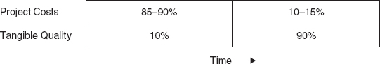
The first 85–90 percent of the budget (i.e., direct labor budget) is needed to generate the first 10 percent of the quality. The last 10–15 percent of the budget often produces the remaining 90 percent of the quality. One does not need an advanced degree in mathematics to realize that a 10 percent cost reduction could easily be accompanied by a 50 percent quality reduction, depending, of course, where the 10 percent was cut.

The following scenario shows the chain of events as they might occur in a typical organization:

• At the beginning of the fiscal year, the executive committee selects those projects to be undertaken, such that all available resources are consumed.
• Shortly into the fiscal year, the executive committee authorizes additional projects that must be undertaken. These projects are added to the queue.
• The executive committee recognizes that the resources available are insufficient to service the queue. Since budgets are tight, hiring additional staff is ruled out. (Even if staff could be hired, the project deadline would be at hand before the new employees were properly trained and up to speed.)
• The executive committee refuses to cancel any of the projects and takes the “easy” way out by adopting the 10 percent solution on each and every project. Furthermore, the executive committee asserts that original performance must be adhered to at all costs.
• Morale in the project and functional areas, which may have taken months to build, is now destroyed overnight. Functional employees lose faith in the ability of the executive committees to operate properly and make sound decisions. Employees seek transfers to other organizations.
• Functional priorities are changed on a daily basis, and resources are continuously shuffled in and out of projects, with very little regard for the schedule.
• As each project begins to suffer, project managers begin to hoard resources, refusing to surrender the people to other projects, even if the work is completed.
• As quality and performance begin to deteriorate, managers at all levels begin writing “protection” memos.
• Schedule and quality slippages become so great that several projects are extended into the next fiscal year, thus reducing the number of new projects that can be undertaken.

The 10 percent solution simply does not work. However, there are two viable alternatives. The first is to use the 10 percent solution, but only on selected projects and after an “impact study” has been conducted, so that the executive committee understands the impact on the time, cost, and performance constraints. The second choice, which is by far the better one, is for the executive committee to cancel or descope selected projects. Since it is impossible to reduce budget without reducing scope, canceling a project or simply delaying it until the next fiscal year is a viable choice. After all, why should all projects have to suffer?

Terminating one or two projects within the queue allows existing resources to be used more effectively, more productively, and with higher organizational morale. However, it does require strong leadership at the executive committee level for the participants to terminate a project rather than to “pass the buck” to the bottom of the organization with the 10 percent solution. Executive committees often function best if the committee is responsible for project selection, prioritization, and tracking, with the middle managers responsible for budgeting.

14.19 LIFE-CYCLE COSTING (LCC)

For years, many R&D organizations have operated in a vacuum where technical decisions made during R&D were based entirely on the R&D portion of the plan, with little regard for what happens after production begins. Today, industrial firms are adopting the life-cycle costing approach that has been developed and used by military organizations. Simply stated, LCC requires that decisions made during the R&D process be evaluated against the total life-cycle cost of the system. As an example, the R&D group has two possible design configurations for a new product. Both design configurations will require the same budget for R&D and the same costs for manufacturing. However, the maintenance and support costs may be substantially greater for one of the products. If these downstream costs are not considered in the R&D phase, large unanticipated expenses may result at a point where no alternatives exist.

Life-cycle costs are the total cost to the organization for the ownership and acquisition of the product over its full life. This includes the cost of R&D, production, operation, support, and, where applicable, disposal. A typical breakdown description might include:

• R&D costs: The cost of feasibility studies; cost-benefit analyses; system analyses; detail design and development; fabrication, assembly, and test of engineering models; initial product evaluation; and associated documentation.
• Production cost: The cost of fabrication, assembly, and testing of production models; operation and maintenance of the production capability; and associated internal logistic support requirements, including test and support equipment development, spare/repair parts provisioning, technical data development, training, and entry of items into inventory.
• Construction cost: The cost of new manufacturing facilities or upgrading existing structures to accommodate production and operation of support requirements.
• Operation and maintenance cost: The cost of sustaining operational personnel and maintenance support; spare/repair parts and related inventories; test and support equipment maintenance; transportation and handling; facilities, modifications, and technical data changes; and so on.
• Product retirement and phaseout cost (also called disposal cost): The cost of phasing the product out of inventory due to obsolescence or wearout, and subsequent equipment item recycling and reclamation as appropriate.

Life-cycle cost analysis is the systematic analytical process of evaluating various alternative courses of action early on in a project, with the objective of choosing the best way to employ scarce resources. Life-cycle cost is employed in the evaluation of alternative design configurations, alternative manufacturing methods, alternative support schemes, and so on. This process includes:

• Defining the problem (what information is needed)
• Defining the requirements of the cost model being used
• Collecting historical data–cost relationships
• Developing estimate and test results

Successful application of LCC will:

• Provide downstream resource impact visibility
• Provide life-cycle cost management
• Influence R&D decision-making
• Support downstream strategic budgeting

There are also several limitations to life-cycle cost analyses. They include:

• The assumption that the product, as known, has a finite life-cycle
• A high cost to perform, which may not be appropriate for low-cost/low-volume production
• A high sensitivity to changing requirements

Life-cycle costing requires that early estimates be made. The estimating method selected is based on the problem context (i.e., decisions to be made, required accuracy, complexity of the product, and the development status of the product) and the operational considerations (i.e., market introduction date, time available for analysis, and available resources).

The estimating methods available can be classified as follows:

• Informal estimating methods
  • Judgment based on experience
  • Analogy
  • SWAG method
  • ROM method
  • Rule-of-thumb method
• Formal estimating methods
  • Detailed (from industrial engineering standards)
  • Parametric

Table 14-14 shows the advantages/disadvantages of each method.

TABLE 14-14. ESTIMATING METHODS

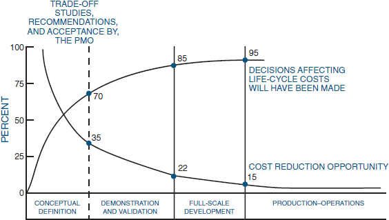
FIGURE 14-16. Department of Defense life-cycle phases.

Figure 14-16 shows the various life-cycle phases for Department of Defense projects. At the end of the demonstration and validation phase (which is the completion of R&D) 85 percent of the decisions affecting the total life-cycle cost will have been made, and the cost reduction opportunity is limited to a maximum of 22 percent (excluding the effects of learning curve experiences). Figure 14-17 shows that, at the end of the R&D phase, 95 percent of the cumulative life-cycle cost is committed by the government. Figure 14-18 shows that, for every $12 that DoD puts into R&D, $28 are needed downstream for production and $60 for operation and support.

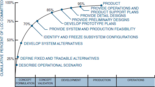
FIGURE 14-17. Actions affecting life-cycle cost (LCC).

FIGURE 14-18. (A) Typical DoD system acquisition LCC profile; (B) typical communication system acquisition LCC profile.

Life-cycle cost analysis is an integral part of strategic planning since today's decision will affect tomorrow's actions. Yet there are common errors made during life-cycle cost analyses:

• Loss or omission of data
• Lack of systematic structure
• Misinterpretation of data
• Wrong or misused techniques
• A concentration on insignificant facts
• Failure to assess uncertainty
• Failure to check work
• Estimating the wrong items

14.20 LOGISTICS SUPPORT

There is a class of projects called “material” projects where the deliverable may require maintenance, service, and support after development. This support will continue throughout the life cycle of the deliverable. Providing service to these deliverables is referred to as logistics support.

In the previous section we showed that approximately 85 percent of the deliverable's life-cycle cost has been committed by the end of the design phase (see Figures 14-16 and 14-17). We also showed that the majority of the total life-cycle cost of a system is in operation and support, and could account for well above 60 percent of the total cost. Clearly, the decisions with the greatest chance of affecting life-cycle cost and identifying cost savings are those influencing the design of the deliverable. Simply stated, proper planning and design can save a company hundreds of millions of dollars once the deliverable is put into use.

The two key parameters used to evaluate the performance of material systems are supportability and readiness. Supportability is the ability to maintain or acquire the necessary human and nonhuman resources to support the system. Readiness is a measure of how good we are at keeping the system performing as planned and how quickly we can make repairs during a shutdown. Clearly, proper planning during the design stage of a project can reduce supportability requirements, increase operational readiness, and minimize or lower logistics support costs.

The ten elements of logistics support include:

• Maintenance planning: The process conducted to evolve and establish maintenance concepts and requirements for the lifetime of a materiel system.
• Manpower and personnel: The identification and acquisition of personnel with the skills and grades required to operate and support a material system over its lifetime.
• Supply support: All management actions, procedures, and techniques used to determine requirements to acquire, catalog, receive, store, transfer, issue, and dispose of secondary items. This includes provisioning for initial support as well as replenishment supply support.
• Support equipment: All equipment (mobile or fixed) required to support the operation and maintenance of a materiel system. This includes associated multiuse end-items; ground-handling and maintenance equipment; tools, metrology, and calibration equipment; and test and automatic test equipment. It includes the acquisition of logistics support for the support and test equipment itself.
• Technical data: Recorded information regardless of form or character (such as manuals and drawings) of a scientific or technical nature. Computer programs and related software are not technical data; documentation of computer programs and related software are. Also other information related to contract administration.
• Training and training support: The processes, procedures, techniques, training devices, and equipment used to train personnel to operate and support a materiel system. This includes individual and crew training; new equipment training; initial, formal, and on-the-job training; and logistic support planning for training equipment and training device acquisitions and installations.
• Computer resource support: The facilities, hardware, software, documentation, manpower, and personnel needed to operate and support embedded computer systems.
• Facilities: The permanent or semipermanent real property assets required to support the materiel system. Facilities management includes conducting studies to define types of facilities or facility improvement, locations, space needs, environment requirements, and equipment.
• Packaging, handling, storage, and transportation: The resources, processes, procedures, design considerations, and methods to ensure that all system, equipment, and support items are preserved, packaged, handled, and transported properly. This includes environmental considerations and equipment preservation requirements for short- and long-term storage and transportability.
• Design interface: The relationship of logistics-related design parameters to readiness and support resource requirements. These logistics-related design parameters are expressed in operational terms rather than as inherent values and specifically relate to system readiness objectives and support costs of the material system.

14.21 ECONOMIC PROJECT SELECTION CRITERIA: CAPITAL BUDGETING

Project managers are often called upon to be active participants during the benefit-to-cost analysis of project selection. It is highly unlikely that companies will approve a project where the costs exceed the benefits. Benefits can be measured in either financial or nonfinancial terms.

The process of identifying the financial benefits is called capital budgeting, which may be defined as the decision-making process by which organizations evaluate projects that include the purchase of major fixed assets such as buildings, machinery, and equipment. Sophisticated capital budgeting techniques take into consideration depreciation schedules, tax information, and cash flow. Since only the principles of capital budgeting will be discussed in this text, we will restrict ourselves to the following topics:

• Payback Period
• Discounted Cash Flow (DCF)
• Net Present Value (NPV)
• Internal Rate of Return (IRR)

14.22 PAYBACK PERIOD

The payback period is the exact length of time needed for a firm to recover its initial investment as calculated from cash inflows. Payback period is the least precise of all capital budgeting methods because the calculations are in dollars and not adjusted for the time value of money. Table 14-15 shows the cash flow stream for Project A.

TABLE 14-15. CAPITAL EXPENDITURE DATA FOR PROJECT A

From Table 14-15, Project A will last for exactly five years with the cash inflows shown. The payback period will be exactly four years. If the cash inflow in Year 4 were $6,000 instead of $5,000, then the payback period would be three years and 10 months.

The problem with the payback method is that $5,000 received in Year 4 is not worth $5,000 today. This unsophisticated approach mandates that the payback method be used as a supplemental tool to accompany other methods.

14.23 THE TIME VALUE OF MONEY

Everyone knows that a dollar today is worth more than a dollar a year from now. The reason for this is because of the time value of money. To illustrate the time value of money, let us look at the following equation:

Using this formula, we can see that an investment of $1,000 today (i.e., PV) invested at 10% (i.e., k) for one year (i.e., n) will give us a future value of $1,100. If the investment is for two years, then the future value would be worth $1,210.

Now, let us look at the formula from a different perspective. If an investment yields $1,000 a year from now, then how much is it worth today if the cost of money is 10%? To solve the problem, we must discount future values to the present for comparison purposes. This is referred to as “discounted cash flows.”

The previous equation can be written as:

Using the data given:

Therefore, $1,000 a year from now is worth only $909 today. If the interest rate, k, is known to be 10%, then you should not invest more than $909 to get the $1,000 return a year from now. However, if you could purchase this investment for $875, your interest rate would be more than 10%.

Discounting cash flows to the present for comparison purposes is a viable way to assess the value of an investment. As an example, you have a choice between two investments. Investment A will generate $100,000 two years from now and investment B will generate $110,000 three years from now. If the cost of capital is 15%, which investment is better?

Using the formula for discounted cash flow, we find that:

PV_A = $75,614

PV_B = $72,327

This implies that a return of $100,000 in two years is worth more to the firm than a $110,000 return three years from now.

14.24 NET PRESENT VALUE (NPV)

The net present value (NPV) method is a sophisticated capital budgeting technique that equates the discounted cash flows against the initial investment. Mathematically,

where FV is the future value of the cash inflows, II represents the initial investment, and k is the discount rate equal to the firm's cost of capital.

Table 14-16 calculates the NPV for the data provided previously in Table 14-15 using a discount rate of 10%.

TABLE 14-16. NPV CALCULATION FOR PROJECT A

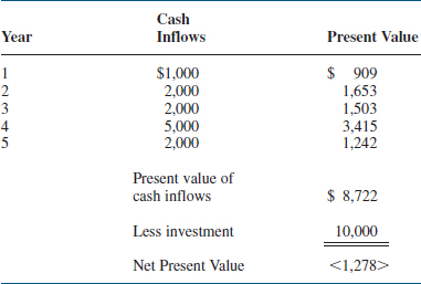
This indicates that the cash inflows discounted to the present will not recover the initial investment. This, in fact, is a bad investment to consider. Previously, we stated that the cash flow stream yielded a payback period of four years. However, using discounted cash flow, the actual payback is greater than five years, assuming that there will be cash inflow in years 6 and 7.

If in Table 14-16 the initial investment was $5,000, then the net present value would be $3,722. The decision-making criteria using NPV are as follows:

• If the NPV is greater than or equal to zero dollars, accept the project.
• If the NPV is less than zero dollars, reject the project.

A positive value of NPV indicates that the firm will earn a return equal to or greater than its cost of capital.

14.25 INTERNAL RATE OF RETURN (IRR)

The internal rate of return (IRR) is perhaps the most sophisticated capital budgeting technique and also more difficult to calculate than NPV. The internal rate of return is the discount rate where the present value of the cash inflows exactly equals the initial investment. In other words, IRR is the discount rate when NPV = 0. Mathematically

The solution to problems involving IRR is basically a trial-and-error solution. Table 14-17 shows that with the cash inflows provided, and with a $5,000 initial investment, an IRR of 10% yielded a value of $3,722 for NPV. Therefore, as a second guess, we should try a value greater than 10% for IRR to generate a zero value for NPV. Table 14-17 shows the final calculation.

The table implies that the cash inflows are equivalent to a 31% return on investment. Therefore, if the cost of capital were 10%, this would be an excellent investment. Also, this project is “probably” superior to other projects with a lower value for IRR.

TABLE 14-17. IRR CALCULATION FOR PROJECT A CASH INFLOWS

TABLE 14-18. CAPITAL PROJECTS

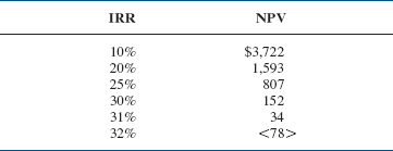
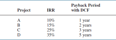
14.26 COMPARING IRR, NPV, AND PAYBACK

For most projects, both IRR and NPV will generate the same accept-reject decision. However, there are differences that can exist in the underlying assumptions that can cause the projects to be ranked differently. The major problem is the differences in the magnitude and timing of the cash inflows. NPV assumes that the cash inflows are reinvested at the cost of capital, whereas IRR assumes reinvestment at the project's IRR. NPV tends to be a more conservative approach.

The timing of the cash flows is also important. Early year cash inflows tend to be at a lower cost of capital and are more predictable than later year cash inflows. Because of the downstream uncertainty, companies prefer larger cash inflows in the early years rather than the later years.

Magnitude and timing are extremely important in the selection of capital projects. Consider Table 14-18.

If the company has sufficient funds for one and only one project, the natural assumption would be to select Project D with a 35% IRR. Unfortunately, companies shy away from long-term payback periods because of the relative uncertainties of the cash inflows after Year 1. One chemical/plastics manufacturer will not consider any capital projects unless the payback period is less than one year and has an IRR in excess of 50%!

14.27 RISK ANALYSIS

Suppose you have a choice between two projects, both of which require the same initial investment, have identical net present values, and require the same yearly cash inflows to break even. If the cash inflow of the first investment has a probability of occurrence of 95% and that of the second investment is 70%, then risk analysis would indicate that the first investment is better.

Risk analysis refers to the chance that the selection of this project will prove to be unacceptable. In capital budgeting, risk analysis is almost entirely based upon how well we can predict cash inflows since the initial investment is usually known with some degree of certainty. The inflows, of course, are based upon sales projections, taxes, cost of raw materials, labor rates, and general economic conditions.

Sensitivity analysis is a simple way of assessing risk. A common approach is to estimate NPV based upon an optimistic (best case) approach, most likely (expected) approach, and pessimistic (worst case) approach. This can be illustrated using Table 14-19. Both Projects A and B require the same initial investment of $10,000, with a cost of capital of 10%, and with expected five-year annual cash inflows of $5,000/year. The range for Project A's NPV is substantially less than that of Project B, thus implying that Project A is less risky. A risk lover might select Project B because of the potential reward of $27,908, whereas a risk avoider would select Project A, which offers perhaps no chance for loss.

TABLE 14-19. SENSITIVITY ANALYSIS

14.28 CAPITAL RATIONING

Capital rationing is the process of selecting the best group of projects such that the highest overall net present value will result without exceeding the total budget available. An assumption with capital rationing is that the projects under consideration are mutually exclusive. There are two approaches often considered for capital rationing.

The internal rate of return approach plots the IRRs in descending order against the cumulative dollar investment. The resulting figure is often called an investment opportunity schedule. As an example, suppose a company has $300,000 committed for projects and must select from the projects identified in Table 14-20. Furthermore, assume that the cost of capital is 10%.

TABLE 14-20. PROJECTS UNDER CONSIDERATION

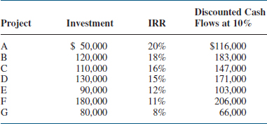
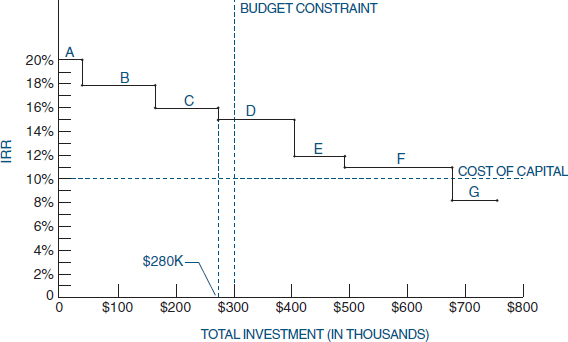
FIGURE 14-19. Investment Opportunity Schedule (IOS) for Table 14-20.

Figure 14-19 shows the investment opportunity schedule. Project G should not be considered because the IRR is less than the firm's cost of capital, but we should select Projects, A, B, and C, which will consume $280,000 out of a total budget of $300,000. This allows us to have the three largest IRRs.

The problem with the IRR approach is that it does not guarantee that the projects with the largest IRRs will maximize the total dollar returns. The reason is that not all of the funds have been consumed.

A better approach is the net present value method. In this method, the projects are again ranked according to their IRRs, but the combination of projects selected will be based upon the highest net present value. As an example, the selection of Projects A, B, and C from Table 14-20 requires an initial investment of $280,000 with resulting discounted cash flows of $446,000. The net present value of Projects A, B, and C is, therefore, $166,000. This assumes that unused portions of the original budget of $300,000 do not gain or lose money. However, if we now select Projects A, B, and D, we will invest $300,000 with a net present value of $170,000 ($470,000 less $300,000). Selection of Projects A, B, and D will, therefore, maximize net present value.

14.29 PROJECT FINANCING²

Project financing involves the establishment of a legally independent project company, usually for large-scale investments (LSI) and long term where the providers of funds are repaid out of cash flow and earnings, and where the assets of the unit (and only the unit) are used as collateral for the loans. Debt repayment would come from the project company only rather than from any other entity. A risk with project financing is that the capital assets may have a limited life. The potential limited life constraint often makes it difficult to get lenders to agree to long-term financial arrangements.

Another critical issue with project financing especially for high-technology projects is that the projects are generally long term. It may be nearly eight to ten years before service will begin, and in terms of technology, eight years can be an eternity. Project financing is often considered a “bet on the future.” And if the project were to fail, the company could be worth nothing after liquidation.

There are several risks that must be considered to understand project financing. The risks commonly considered are

Financial Risks

• Use of project versus corporate financing
• Use of corporate bonds, stock, zero coupon bonds, and bank notes
• Use of secured versus unsecured debt
• The best sequence or timing for raising capital
• Bond rating changes
• Determination of the refinancing risk, if necessary

Development Risks

• Reality of the assumptions
• Reality of the technology
• Reality of development of the technology
• Risks of obsolescence

Political Risks

• Sovereignty risks
• Political instability
• Terrorism and war
• Labor availability
• Trade restrictions
• Macroeconomics such as inflation, currency conversion, and transferability of funding and technology

Organizational Risks

• Members of the board of directors
• Incentives for the officers
• Incentives for the board members
• Bonuses as a percentage of base compensation
• Process for the resolution of disputes

Execution Risks

• Timing when execution will begin
• Life expectancy of execution
• Ability to service debt during execution

14.30 STUDYING TIPS FOR THE PMI^® PROJECT MANAGEMENT CERTIFICATION EXAM

This section is applicable as a review of the principles to support the knowledge areas and domain groups in the PMBOK^® Guide. This chapter addresses:

• Integration Management
• Scope Management
• Time Management
• Cost Management
• Initiating
• Planning

Understanding the following principles is beneficial if the reader is using this text to study for the PMP^® Certification Exam:

• What is meant by cost-estimating relationships (CER)
• Three basic types of estimates
• Relative accuracy of each type of estimate and the approximate time to prepare the estimate
• Information that is needed to prepare the estimates (i.e., labor, material, overhead rates, etc.)
• Importance of backup data for costs
• Estimating pitfalls
• Concept of rolling wave planning
• What is meant by life cycle costing
• Different ways of evaluating a project's financial feasibility or benefits (i.e., ROI, payback period, net present value, internal rate of return, depreciation, scoring models)

The following multiple-choice questions will be helpful in reviewing the principles of this chapter:

1. Which of the following is a valid way of evaluating the financial feasibility of a project?
   1. Return on investment
   2. Net present value
   3. Internal rate of return
   4. All of the above
2. The three common classification systems for estimates includes all of the following except:
   1. Parametric estimates
   2. Quick-and-dirty estimates
   3. Analogy estimates
   4. Engineering estimates
3. The most accurate estimates are:
   1. Parametric estimates
   2. Quick-and-dirty estimates
   3. Analogy estimates
   4. Engineering estimates
4. Which of the following is considered to be a bottom-up estimate rather than a top-down estimate?
   1. Parametric estimates
   2. Analogy estimates
   3. Engineering estimates
   4. None of the above
5. Which of the following would be considered as a cost-estimating relationship (CER)?
   1. Mathematical equations based upon regression analysis
   2. Learning curves
   3. Cost–cost or cost–quantity relationships
   4. All of the above
6. If a worker earns $30 per hour in salary but the project is charged $75 per hour for each hour the individual works, then the overhead rate is:
   1. 100%
   2. 150%
   3. 250%
   4. None of the above
7. Information supplied to a customer to support the financial data provided in a proposal is commonly called:
   1. Backup data
   2. Engineering support data
   3. Labor justification estimates
   4. Legal rights estimates
8. Estimating pitfalls can result from:
   1. Poorly defined statement of work
   2. Failure to account for risks in the estimates
   3. Using the wrong estimating techniques
   4. All of the above
9. The source of many estimating risks is:
   1. Poorly defined requirements
   2. An inexperienced project manager
   3. Lack of management support during estimating
   4. All of the above
10. A project where the scope evolves as the work takes place is called either progressive planning or:
    1. Synchronous planning
    2. Continuous planning
    3. Rolling wave planning
    4. Continuous reestimation planning
11. The calculation of the total cost of a product, from R&D to operational support and disposal, is called:
    1. Birth-to-death costing
    2. Life-cycle costing
    3. Summary costing
    4. Depreciation costing

ANSWERS

1. D
2. B
3. D
4. C
5. D
6. B
7. A
8. D
9. D
10. C
11. B

PROBLEMS

14–1 How does a project manager price out a job in which the specifications are not prepared until the job is half over?

14–2 Beta Corporation is in the process of completing a contract to produce 150 units for a given customer. The contract consisted of R&D, testing and qualification, and full production. The industrial engineering department had determined that the following number of hours were required to produce certain units:

1. Plot the data points on regular graph paper with the Y-axis as hours and the X-axis as number of units produced.
2. Plot the data points on log–log paper and determine the slope of the line.
3. Compare parts a and b. What are your conclusions?
4. How much time should it take to manufacture the 150th unit?
5. How much time should it take to manufacture the 1,000th unit? Explain your answer. Is it realistic? If not, why?
6. As you are producing the 150th unit, you receive an immediate follow-on contract for another 150 units. How many manufacturing hours should you estimate for the follow-on effort (using only the learning curves)?
7. Let's assume that industrial engineering determines that the optimum number of hours (for 100 percent efficiency) of manufacturing is forty-five. At what efficiency factor are you now performing at the completion of unit number 150? After how many units in the follow-on contract will you reach the optimum level?
8. At the end of the first follow-on contract, your team and personnel are still together and performing at a 100 percent efficiency position (of part g). You have been awarded a second follow-on contract, but the work will not begin until six months from now. Assuming that you can assemble the same team, how many man-hours/unit will you estimate for the next 150-unit follow-on?
9. Would your answer to part h change if you could not assemble the same team? Explain your answer quantitatively.
10. You are now on the contract negotiation team for the second follow-on contract of 150 units (which is not scheduled to start for six months). Based on the people available and the “loss of learning” between contracts, your industrial engineering department estimates that you will be performing at a 60 percent efficiency factor. The customer says that your efficiency factor should be at least 75 percent. If your company is burdened at $40/hour, how much money is involved between the 60 and 75 percent efficiency factors?
11. What considerations should be made in deciding where to compromise in the efficiency factor?

14–3 With reference to Figure 14-10, under what conditions could each of the following situations occur:

1. Program manager and program office determine labor hours by pricing out the work breakdown structure without coordination with functional management.
2. Upper-level management determines the price of a bid without forming a program office or consulting functional management.
3. Perturbations on the base case are not performed.
4. The chief executive officer selects the program manager without consulting his directors.
5. Upper-level management does not wish to have a cost review meeting prior to submittal of a bid.

14–4 Can Figure 14-20 be used effectively to price out the cost of preparing reports?

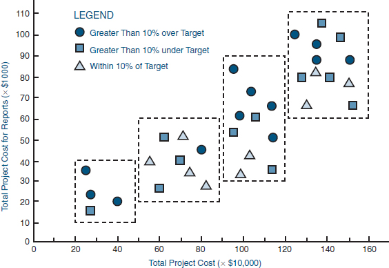
FIGURE 14-20. Project documentation costs.

14–5 Answer the following questions with reference to Figure 14-10.

1. The base case for a program is priced out at $22 million. The company's chief executive officer is required to obtain written permission from corporate to bid on programs in excess of $20 million. During the price review meeting the chief executive states that the bid will be submitted at $19.5 million. Should you, as program manager, question this?
2. Would your answer to part a change if this program were a follow-on to an earlier program?
3. Proposals normally consist of management, technical, and cost volumes. Indicate in Figure 14-10 where these volumes can go to press, assuming each can be printed independently.

14–6 Under what kind of projects would each of the following parameters be selected:

1. Salary escalation factor of 0 percent.
2. Material termination liability of 0 percent or 100 percent.
3. Material commitments for twenty months of a twenty-four-month program.
4. Demanning ratio of 0 percent or 100 percent of following months' labor.

14–7 How can upper-level management use the functional cost and hour summary to determine manpower planning for the entire company? How would you expect management to react if the functional cost and hour summary indicated a shortage or an abundance of trained personnel?

14–8 Which of the figures presented in this chapter should program management make available to the functional managers? Explain your answer.

14–9 The Jennings Construction Company has decided to bid on the construction for each of the two phases of a large project. The bidding requirements are that the costs for each phase be submitted separately together with a transition cost for turning over the first phase of the program to a second contractor should Jennings not receive both awards or perform unsatisfactorily on the first phase. The evaluation for the award of the second phase will not be made until the first phase is near completion. How can the transition costs be identified in the strategic planning model?

14–10 Two contractors decide to enter into a joint venture on a project. What difficulties can occur if the contractors have decided on who does what work, but changes may take place if problems occur? What happens if one contractor has higher salary levels and overhead rates?

14–11 The Jones Manufacturing Company is competing for a production contract that requires that work begin in January 2003. The cost package for the proposal must be submitted by July 2002. The business base, and therefore the overhead rates, are uncertain because Jones has the possibility of winning another contract, to be announced in September 2002. How can the impact of the announcement be included in the proposal? How would you handle a situation where another contract may not be renewed after January 2003, i.e., assume that the announcement would not be made until March?

14–12 Many competitive programs contain two phases: research and development, and production. Production profits far exceed R&D profits. The company that wins the R&D contract normally becomes a favorite for the production contract, as well as for any follow-on work. How can the dollar figures attached to follow-on work influence the cost package that you submit for the R&D phase? Would your answer change if the man-hours submitted for the R&D phase become the basis for the production phase?

14–13 During initial pricing activities, one of the functional managers discovers that the work breakdown structure requires costing data at a level that is not normally made, and will undoubtedly incur additional costs. How should you, as a program manager, respond to this situation? What are your alternatives?

14–14 Should the project manager give the final manpower loading curves to the functional managers? If so, at what point in time?

14–15 You have been asked to price out a project for an outside customer. The project will run for eight months. Direct labor is S100,000 for each month and the overhead rate is fixed at 100 percent per month. Termination liability on the direct labor and overhead rate is 80 percent of the following month's expenses. Material expenses are as follows:

Material A: Cost is $100,000 payable 30 days net. Material is needed at the end of the fifth month. Lead time is four months with termination liability expenses as follows:

30 days: 25%

60 days: 75%

90 days: 100%

Material B: Cost is $200,000, payable on delivery. Material is needed at the end of the seventh month. Lead time is three months with termination liability as follows:

30 days: 50%

60 days: 100%

Complete the table below, neglecting profits.

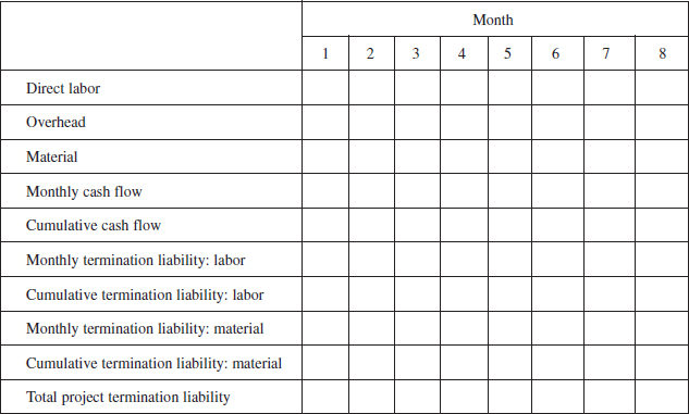
14–16 Should a project manager be appointed in the bidding stage of a project? If so, what authority should he have, and who is responsible for winning the contract?

14–17 Explain how useful each of the following can be during the estimating of project costs:

1. Contingency planning and estimating
2. Using historical databases
3. Usefulness of computer estimating
4. Usefulness of performance factors to account for inefficiencies and uncertainties.