Chapter 1
Working with Numbers, Text, and Dates
IN THIS CHAPTER
![]() Mastering whole numbers
Mastering whole numbers
![]() Juggling numbers with decimal points
Juggling numbers with decimal points
![]() Simplifying strings
Simplifying strings
![]() Conquering Boolean True/False
Conquering Boolean True/False
![]() Working with dates and times
Working with dates and times
Computer languages in general, and certainly Python, deal with information in ways that are different from what you may be used to in your everyday life. This idea takes some getting used to. In the computer world, numbers are numbers you can add, subtract, multiply, and divide. Python also differentiates between whole numbers (integers) and numbers that contain a decimal point (floats). Words (textual information such as names and addresses) are stored as strings, which is short for “a string of characters.” In addition to numbers and strings, there are Boolean values, which can be either True or False.
In real life, we also have to deal with dates and times, which are yet another type of information. Python doesn't have a built-in data type for dates and times, but thankfully, a free module you can import any time works with such information. This chapter is all about taking full advantage of the various Python data types.
Calculating Numbers with Functions
A function in Python is similar to a function on a calculator, in that you pass something into the function, and the function passes something back. For example, most calculators and programming languages have a square root function: You give them a number, and they give back the square root of that number.
Python functions generally have the syntax:
variablename = functioname(param[,param])
Because most functions return some value, you typically start by defining a variable to store what the function returns. Follow that with the = sign and the function name, followed by a pair of parentheses. Inside the parentheses you may pass one or more values (called parameters) to the function.
For example, the abs() function accepts one number and returns the absolute value of that number. If you're not a math nerd, this just means if you pass it a negative number, it returns that same number as a positive number. If you pass it a positive number, it returns the same number you passed it. In other words, the abs() function simply converts negative numbers to positive numbers.
As an example, in Figure 1-1 (which you can try out for yourself hands-on in a Jupyter notebook, at the Python prompt, or in a .py file in VS Code), we created a variable named x and assigned it the value -4. Then we created a variable named y and assigned it the absolute value of x using the abs() function. Printing x shows its value, -4, which hasn't changed. Printing y shows 4, the absolute value of x as returned by the abs() function.

FIGURE 1-1: Trying out the abs() function.
Even though a function always returns one value, some functions accept two or more values. For example, the round() function takes one number as its first argument. The second argument is the number of decimal places to which you want to round that number, for example, 2 for two decimal places. In the example in Figure 1-2, we created a variable, x, with a whole lot of digits after the decimal point. Then we created a variable named y to return the same number rounded to two decimal places. Then we printed both results.

FIGURE 1-2: Trying out the round() function.
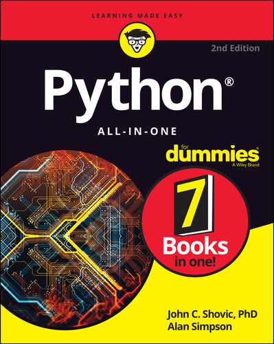
Python has many built-in functions for working with numbers, as shown in Table 1-1. Some may not mean much to you if you're not into math in a big way, but don't let that intimidate you. If you don't understand what a function does, chances are it's not doing something relevant to the kind of work you do. But if you're curious, you can always search the web for python followed by the function name for more information. For a more extensive list, search for python 3 built-in functions.
TABLE 1-1 Some Built-In Python Functions for Numbers
Built-In Function |
Purpose |
|---|---|
|
Returns the absolute value of number x (converts negative numbers to positive). |
|
Returns a string representing the value of x converted to binary. |
|
Converts a string or number x to the float data type. |
|
Returns x formatted according to the a pattern specified in y. This older syntax has been replaced with f-strings in current Python versions. |
|
Returns a string containing x converted to hexadecimal, prefixed with 0x. |
|
Converts x to the integer data type by truncating (not rounding) the decimal portion and any digits after it. |
|
Takes any number of numeric arguments and returns whichever is the largest. |
|
Takes any number of numeric arguments and returns whichever is the smallest. |
|
Converts x to an octal number, prefixed with 0o to indicate octal. |
|
Rounds the number x to y number of decimal places. |
|
Converts the number x to the string data type. |
|
Returns a string indicating the data type of x. |
Figure 1-3 shows examples of proper Python syntax for using the built-in math functions.
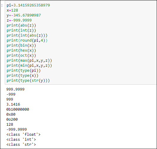
FIGURE 1-3: Playing around with built-in math functions at the Python prompt.
You can also nest functions — meaning you can put functions inside functions. For example, when z = -999.9999, the expression print(int(abs(z))) prints the integer portion of the absolute value of z, which is 999. The original number is converted to positive, and then the decimal point and everything to its right chopped off.
Still More Math Functions
In addition to the built-in functions you've learned about so far, still others you can import from the math module. If you need them in an app, put import math.py file or Jupyter cell to make those functions available to the rest of the code. Or to use them at the command prompt, first enter the import math command.
One of the functions in the math module is the sqrt() function, which gets the square root of a number. Because it's part of the math module, you can't use it without importing the module first. For example, if you enter the following, you'll get an error because sqrt() isn't a built-in function:
print(sqrt(81))
Even if you do two commands like the following, you'll still get an error because you're treating sqrt() as a built-in function:
import math
print(sqrt(81))
To use a function from a module, you have to import the module and precede the function name with the module name and a dot. So let's say you have some value, x, and you want the square root. You have to import the math module and use math.sqrt(x) to get the correct answer, as shown in Figure 1-4. Entering that command shows 9.0 as the result, which is indeed the square root of 81.
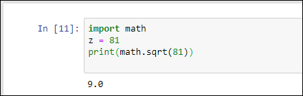
FIGURE 1-4: Using the sqrt() function from the math module.
The math module offers a lot of trigonometric and hyperbolic functions, powers and logarithms, angular conversions, constants such as pi and e. We won't delve into all of them because advanced math isn’t relevant to most people. You can check them all out anytime by searching the web for python 3 math module functions. Table 1-2 offers examples that may prove useful in your own work.
TABLE 1-2 Some Functions from the Python Math Module
Built-In Function |
Purpose |
|---|---|
|
Returns the arccosine of |
|
Returns the arctangent of |
|
Converts rectangular coordinates (x, y) to polar coordinates (r, theta) |
|
Returns the ceiling of |
|
Returns the cosine of |
|
Converts angle |
|
Returns the mathematical constant e (2.718281 …) |
|
Returns e raised to the power x, where e is the base of natural logarithms |
|
Returns the factorial of |
|
Returns the floor of |
|
Returns |
|
Returns the logarithm of |
|
Returns the base-2 logarithm of |
|
Returns the mathematical constant pi (3.141592 …) |
|
Returns |
|
Converts angle |
|
Returns the sine of |
|
Returns the square root of x |
|
Returns the tangent of |
|
Returns the mathematical constant tau (6.283185 …) |
The constants pi, e, and tau are unusual for functions in that you don't use parentheses. As with any function, you can use these functions in expressions (calculations) or assign their values to variables. Figure 1-5 shows some examples of using functions from the math module.

FIGURE 1-5: More playing around with built-in math functions at the Python prompt.
Formatting Numbers
Over the years, Python has offered different methods for displaying numbers in formats familiar to us humans. For example, most people would rather see dollar amounts expressed in the format $1,234.56 rather than 1234.560065950695405695405959. The easiest way to format numbers in Python, starting with version 3.6, is to use f-stings.
Formatting with f-strings
Format strings, or f-strings, are the easiest way to format data in Python. All you need is a lowercase f or uppercase F followed immediately by some text or expressions enclosed in quotation marks. Here is an example:
f"Hello {username}"
The f before the first quotation mark tells Python that what follows is a format string. Inside the quotation marks, the text, called the literal part, is displayed literally (exactly as typed in the f-string). Anything in curly braces is the expression part of the f-string, a placeholder for what will appear when the code executes. Inside the curly braces, you can have an expression (a formula to perform some calculation, a variable name, or a combination of the two). Here is an example:
username = "Alan"
print(f"Hello {username}")
When you run this code, the print function displays the word Hello, followed by a space, followed by the contents of the username variable, as shown in Figure 1-6.
FIGURE 1-6: A super simple f-string for formatting.
Here is another example of an expression — the formula quantity times unit_price — inside the curly braces:
unit_price = 49.99
quantity = 30
print(f"Subtotal: ${quantity * unit_price}")
The output from that, when executed, follows:
Subtotal: $1499.7
That $1499.7 isn't an ideal way to show dollar amounts. Typically, we like to use commas in the thousands places, and two digits for the pennies, as in the following:
Subtotal: $1,499.70
Fortunately, f-strings provide you with the means to do this formatting, as you learn next.
Showing dollar amounts
To get a comma to appear in the dollar amount and the pennies as two digits, you can use a format string inside the curly braces of an expression in an f-string. The format string starts with a colon and needs to be placed inside the closing curly brace, right up against the variable name or the value shown.
To show commas in thousands places, use a comma in your format string right after the colon, like this:
:,
Using the current example, you would do the following:
print(f"Subtotal: ${quantity * unit_price:,}")
Executing this statement produces this output:
Subtotal: $1,499.7
To get the pennies to show as two digits, follow the comma with
.2f
The .2f means “two decimal places, fixed” (never any more or less than two decimal places). The following code will display the number with commas and two decimal places:
print(f"Subtotal: ${quantity * unit_price:,.2f}")
Here's what the code displays when executed:
Subtotal: $1,499.70
Perfect! That's exactly the format we want. So anytime you want to show a number with commas in the thousands places and exactly two digits after the decimal point, use an f-string with the format string, .2f.
Formatting percent numbers
Now, suppose your app applies sales tax. The app needs to know the sales tax rate, which should be expressed as a decimal number. So if the sales tax rate is 6.5 percent, it has to be written as 0.065 (or .065, if you prefer) in your code, like this:
sales_tax_rate = 0.065
It's the same amount with or without the leading zero, so just use whichever format works for you.
This number format is ideal for Python, and you wouldn't want to mess with that. But if you want to display that number to a human, simply using a print() function displays it exactly as Python stores it:
sales_tax_rate = 0.065
print(f"Sales Tax Rate {sales_tax_rate}")
Sales Tax Rate 0.065
When displaying the sales tax rate for people to read, you'll probably want to use the more familiar 6.5% format rather than .065. You can use the same idea as with fixed numbers (.2f). However, you replace the f for fixed numbers with %
print(f"Sales Tax Rate {sales_tax_rate:.2%}")
Running this code multiples the sales tax rate by 100 and follows it with a % sign, as you can see in Figure 1-7.

FIGURE 1-7: Formatting a percentage number.
In both of the previous examples, we used 2 for the number of digits. But of course you can display any number of digits you want, from zero (none) to whatever level of precision you need. For example, using .1%
print(f"Sales Tax Rate {sales_tax_rate:.1%}")
displays this output when the line is executed:
Sales Tax Rate 6.5%
Replacing 1 with a 9, like this:
print(f"Sales Tax Rate {sales_tax_rate:.9%}")
displays the percentage with nine digits after the decimal point:
Sales Tax Rate 6.500000000%
You don't need to use an f-string only inside a call to the print function. You can also execute an f-string and save the result in a variable that you can display later. The format string itself is like any other string in that it must be enclosed in single, double, or triple quotation marks. When using triple quotation marks, you can use either three single quotation marks or three double quotation marks. It doesn't matter which you use as the outermost quotation marks on the format string; the output is the same, as you can see in Figure 1-8.
 For single and double quotation marks, use the corresponding keyboard keys. For triple quotation marks, you can use three of either. Make sure you end the string with exactly the same characters you used to start the string. For example, all the strings in Figure 1-8 are perfectly valid code, and they will all be treated the same.
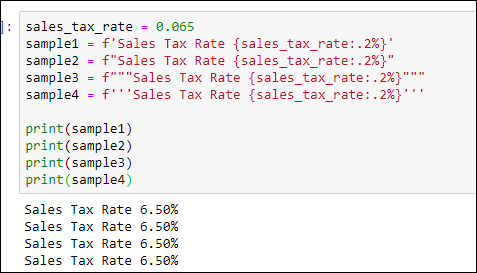
FIGURE 1-8: An f-string can be encased in single, double, or triple quotation marks.
Making multiline format strings
If you want to have multiline output, you can add line breaks to your format strings in a few ways:
- Use
/n: You can use a single-line format string withuser1 = "Alberto"
user2 = "Babs"
user3 = "Carlos"
output=f"{user1} {user2} {user3}"
print(output)When executed, this code displays:
Alberto
Babs
Carlos - Use triple quotation marks (single or double): If you use triple quotation marks around your format string, you don't need to use

FIGURE 1-9: A multiline f-string enclosed in triple quotation marks.
As you can see, the output honors the line breaks and even the blank spaces in the format string. Unfortunately, it's not perfect — in real life, we would right align the numbers so that the decimal points line up. All is not lost, though, because with format strings you can also control the width and alignments of your output.
Formatting width and alignment
You can also control the width of your output (and the alignment of content within that width) by following the colon in your f-string with < (for left aligned), ^ (for centered), or > (for right aligned). Put any of these characters right after the colon in your format string. For example, the following will make the output 20 characters wide, with the content right aligned:
:>20
In Figure 1-9, all the dollar amounts are left aligned, because that's the default. To right align numbers, which is how we usually see dollar amounts, you can use > in an f-string. To make the numbers the same width, specify a number after the > character. For example, in Figure 1-10, each f-string includes >9, which causes each displayed number to be right aligned and 9 characters wide. The output, which you can see at the bottom of the figure, makes all the numbers align to the right, with their dollar signs neatly aligned to the left. The spaces to the right of each dollar sign make sure each number is exactly 9 characters wide.

FIGURE 1-10: All dollar amounts are right aligned within a width of 9 characters (>9).
You may look at Figure 1-10 and wonder why the dollar signs are lined up the way they are. Why aren't they aligned right next to their numbers? The dollar signs are part of the literal string, outside the curly braces, so they aren't affected by the >9 inside the curly braces.
Realigning the dollar signs is a little more complicated than you might imagine, because you can use the ,.2f formatting only on a number. You can't attach a $ to the front of a number unless you change the number to a string — but then it wouldn't be a number anymore, so.2f wouldn't work.
But complicated doesn't mean impossible; it just means inconvenient. You can convert each dollar amount to a string in the current format, stick the dollar sign on that string, and then format the width and alignment on this string. For example, the following code creates a variable named s-subtotal containing a dollar sign immediately followed by the dollar amount, with the dollar sign just to the left of the first digit and no spaces after the dollar sign:
s_subtotal = "$" + f"{subtotal:,.2f}"
In this code, we assume the subtotal variable contains some number. Let's say the number is 1598.402, though it could be any number. The f"{subtotal:,2f}" formats the number in a fixed two-decimal-places format with a comma in the thousands place, like this:
1,598.40
The output is a string rather than a number because an f-string always produces a string.
The following part of the code sticks (concatenates) a dollar sign in the front:
"$"+
So now the output is $1,598.40. That final formatted string is stored in a new variable named s_subtotal. (We added the leading s_ to remind us that this is the string equivalent of the subtotal number, not the original number.)
To display that dollar amount right aligned with a width of 9 digits, use >9 in a new format string to display the s_subtotal variable, like this:
f{s_subtotal:>9}
 When you use
 + with strings, you concatenate (join) the two strings. The + only does addition with numbers, not strings.
Figure 1-11 shows a complete example, including the output from running the code. All the numbers are right aligned with the dollar signs in the usual place.
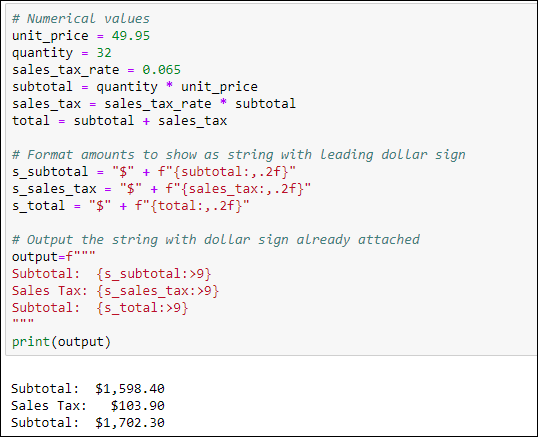
FIGURE 1-11: All the dollar amounts neatly aligned.
Grappling with Weirder Numbers
Most of us deal with simple numbers like quantities and dollar amounts all the time. If your work requires you to deal with bases other than 10 or imaginary numbers, Python has the stuff you need to do the job. But keep in mind that you don't need to learn these things to use Python or any other language. You would use these only if your actual work (or perhaps homework) requires it. In the next section, you look at some number types commonly used in computer science: binary, octal, and hexadecimal numbers.
Binary, octal, and hexadecimal numbers
If your work requires dealing with base 2, base 8, or base 16 numbers, you're in luck because Python has symbols for writing these as well as functions for converting among them. Table 1-3 shows the three non-decimal bases and the digits used by each.
TABLE 1-3 Python for Base 2, 8, and 16 Numbers
System |
Also Called |
Digits Used |
Symbol |
Function |
|---|---|---|---|---|
Base 2 |
Binary |
0,1 |
0b |
|
Base 8 |
Octal |
0,1,2,3,4,5,6,7 |
0o |
|
Base 16 |
Hexadecimal or hex |
0,1,2,3,4,5,6,7,8,9, A,B,C,D,E,F |
0x |
|
Most people never have to work with binary, octal, or hexadecimal numbers. So if all of this is giving you the heebie-jeebies, don't sweat it. If you’ve never heard of them before, chances are you’ll never hear of them again after you’ve completed this section.
If you want more information about the various numbering systems, you can use your favorite search engine to search for binary number or octal, or decimal, or hexadecimal.
You can use these various functions to convert how the number is displayed at the Python prompt, of course, as well as in an apps you create. At the prompt, just use the print() function with the conversion function inside the parentheses, and the number you want to convert inside the innermost parentheses. For example, the following displays the hexadecimal equivalent of the number 255:
print(hex(255))
The result is 0xff, where the 0x indicates that the number that follows is expressed in hex, and ff is the hexadecimal equivalent of 255.
To convert from binary, octal, or hex to decimal, you don't need to use a function. Just use print() with the number you want to convert inside the parentheses. For example, print(0xff) displays 255, the decimal equivalent of hex ff. Figure 1-12 shows some more examples you can try at the Python prompt.

FIGURE 1-12: Messing about with binary, octal, and hex.
Complex numbers
Complex numbers are another one of those weird numbering things you may never have to deal with unless you happen to be into electrical engineering, higher math, or a branch of science that uses them. A complex number is one that can be expressed as a+bi where a and b are real numbers, and i represents the imaginary number satisfied by the equation x2=–1. There is no real number x whose square equals –1, so that's why it’s called an imaginary number.
Some branches of math use a lowercase i to indicate an imaginary number. But Python uses j (as do those in electrical engineering because i is used to indicate current).
Anyway, if your application requires working with complex numbers, you can use the complex() function to generate an imaginary number, using the following syntax:
complex(real,imaginary)
Replace real with the real part of the complex number, and replace imaginary with the imaginary number. For example, in code or the command prompt, try this:
z = complex(2,-3)
The variable z gets the imaginary number 2–3j. Then use a print() function to display the contents of z, like this:
print(z)
The screen displays the imaginary number 2-3j.
You can tack .real or .imag onto an imaginary number to get the real or imaginary part. For example, the following produces 2.0, which is the real part of the number z:
print(z.real)
And this returns –3.0, which is the imaginary part of z:
print(z.imag)
Once again, if none of this makes sense to you, don't worry. It’s not required for learning or doing Python. Python simply offers complex numbers and these functions for people who happen to require them.
 If your work requires working with complex numbers, search the web for python cmath to learn about Python's
 cmath module, which provides functions for complex numbers.
Manipulating Strings
In Python and other programming languages, we refer to words and chunks of text as strings, short for “a string of characters.” A string has no numeric meaning or value. (We discuss the basics of strings in Book 1, Chapter 4.) In this section, you learn Python coding skills for working with strings.
Concatenating strings
You can join strings by using a + sign. The process of doing so is called string concatenation in nerd-o-rama world. One thing that catches beginners off-guard is the fact that a computer doesn't know a word from a bologna sandwich. So when you join strings, the computer doesn't automatically put spaces where you'd expect them. For example, in the following code, full_name is a concatenation of the first three strings.
first_name = "Alan"
middle_init = "C"
last_name = "Simpson"
full_name = first_name+middle_init + last_name
print(full_name)
When you run this code to print the contents of the full_name variable, you can see that Python did join them in one long string:
AlanCSimpson
Nothing is wrong with this output, per se, except that we usually put spaces between words and the parts of a person's name.
Because Python won’t automatically put in spaces where you think they should go, you have to put them in yourself. The easiest way to represent a single space is by using a pair of quotation marks with one space between them, like this:
" "
If you forget to put the space between the quotation marks, like the following, you won't get a space in your string because there's no space between the quotation marks:
""
You can put multiple spaces between the quotation marks if you want multiple spaces in your output, but typically one space is enough. In the following example, you put a space between first_name and last_name. You also stick a period and space after middle_init:
first_name = "Alan"
middle_init = "C"
last_name = "Simpson"
full_name = first_name + " " + middle_init + ". " + last_name
print(full_name)
The output of this code, which is the contents of that full_name variable, looks more like the kind of name you're used to seeing:
Alan C. Simpson
Getting the length of a string
To determine how many characters are in a string, you use the built-in len() function (short for length). The length includes spaces because spaces are characters, each one having a length of one. An empty string — that is, a string with nothing in it, not even a space — has a length of zero.
Here are some examples. In the first line you define a variable named s1 and put an empty string in it (a pair of quotation marks with nothing in between). The s2 variable gets a space (a pair of quotation marks with a space between). The s3 variable gets a string with some letters and spaces. Then, three print() functions display the length of each string:
s1 = ""
s2 = " "
s3 = "A B C"
print(len(s1))
print(len(s2))
print(len(s3))
Following is the output from that code, when executed. The output makes perfect sense when you understand that len() measures the length of strings as the number of characters (including spaces) in the string:
0
1
5
Working with common string operators
Python offers several operators for working with sequences of data. One weird thing about strings in Python (and in most other programming languages) is that when you're counting characters, the first character counts as 0, not 1. This makes no sense to us humans. But computers count characters that way because it’s the most efficient method. So even though the string in Figure 1-13 is five characters long, the last character in that string is the number 4, because the first character is number 0. Go figure.

FIGURE 1-13: Character positions in a string start at 0, not 1.
Table 1-4 summarizes the Python 3 operators for working with strings.
TABLE 1-4 Python Sequence Operators That Work with Strings
Operator |
Purpose |
|---|---|
|
Returns |
|
Returns |
|
Repeats string |
|
The |
|
A slice from string |
|
A slice of |
|
The smallest (lowest) character of string |
|
The largest (highest) character of string |
|
The numeric position of the first occurrence of |
|
The number of times string |
Figure 1-14 shows examples of using the string operators in Jupyter Notebook. When the output of a print() function doesn't look right, keep in mind two important facts about strings in Python:
- The first character is always number
0. - Every space counts as one character, so don't skip spaces when counting.

FIGURE 1-14: Playing around with string operators in Jupyter Notebook.
You may have noticed that min(s) returns a blank space, meaning that the blank space character is the lowest character in that string. But what exactly makes the space “lower” than the letter A or the letter a? The simple answer is the letter's ASCII number. Every character you can type at your keyboard, and many additional characters, have a number assigned by the American Standard Code for Information Interchange (ASCII).
Figure 1-15 shows a chart with ASCII numbers for many common characters. Spaces and punctuation characters are “lower” than A because they have smaller ASCII numbers. Uppercase letters are “lower” than lowercase letters because they have smaller ASCII numbers. Are you wondering what happened to the characters assigned to numbers 0–31? These numbers have characters too, but they are control characters and are essentially non-printing and invisible, such as when you hold down the Ctrl key and press another key.
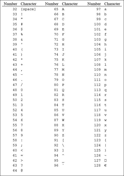
FIGURE 1-15: ASCII numbers for common characters.
Python offers two functions for working with ASCII. The ord() function takes a character as input and returns the ASCII number of that character. For example, print(ord("A")) returns 65, because an uppercase A is character 65 in the ASCII chart. The chr() function does the opposite. You give it a number, and it returns the ASCII character for that number. For example, print(chr(65)) displays A because A is character 65 in the ASCII chart.
Manipulating strings with methods
Every string in Python 3 is considered a str object (pronounced “string object”). The shortened word str for string distinguishes Python 3 from earlier versions of Python, which referred to string as string objects (with the word string spelled out, not shortened). This naming convention is a great source of confusion, especially for beginners. Just try to remember that in Python 3, str is all about strings of characters.
Python offers numerous str methods (also called string methods) to help you work with str objects. The general syntax of str object methods is as follows:
string.methodname(params)
where string is the string you're analyzing, methodname is the name of a method from Table 1-5, and params refers to any parameters that you need to pass to the method (if required). The leading s in the first column of Table 1-5 means “any string,” be it a literal string enclosed in quotation marks or the name of a variable that contains a string.
TABLE 1-5 Built-In Methods for Python 3 Strings
Method |
Purpose |
|---|---|
|
Returns a string with the first letter capitalized and the rest lowercase. |
|
Returns the number of times string |
|
Returns a number indicating the first position at which string |
|
Similar to |
|
Returns |
|
Returns |
|
Returns |
|
Returns |
|
Returns |
|
Returns |
|
Returns |
|
Returns |
|
Returns |
|
Returns a copy of string |
|
Similar to |
|
Same as |
|
Returns string |
|
Returns string |
|
Returns string |
|
Returns string |
|
Returns string |
You can play around with these methods in a Jupyter notebook, at the Python prompt, or in a .py file. Figure 1-16 shows some examples in a Jupyter notebook using three variables named s1, s2, and s3 as strings to experiment with. The result of running the code appears below the code.

FIGURE 1-16: Playing around with Python 3 string functions.
Don't bother trying to memorize or even make sense of every string method. Remember instead that if you need to operate on a string in Python, you can do a web search for python 3 string methods to find out what's available.
Uncovering Dates and Times
In the world of computers, we often use dates and times for scheduling, or for calculating when something is due or how many days it's past due. We sometimes use timestamps to record exactly when a user did something or when an event occurred. There are lots of reasons for using dates and times in Python, but perhaps surprisingly, no built-in data type for them exists like the ones for strings and numbers.
To work with dates and times, you typically need to use the datetime module. Like any module, you must import it before you can use it. You do that using import datetime. As with any import, you can add an alias (nickname) that's easier to type, if you like. For example, import datetime as dt would work too. You just have to remember to type dt rather than datetime in your code when calling upon the capabilities of that module.
The datetime module is an abstract base class, which is a fancy way of saying it offers new data types to the language. For dates and times, those data types are as follows:
datetime.date: A date consisting of month, day, and year (but no time information).datetime.time: A time consisting of hour, minute, second, microsecond, and optionally time zone information if needed (but no date).datetime.datetime: A single item of data consisting of date, time, and optionally time zone information.
We preceded each type with the full word datetime in the preceding list, but if you use an alias, such as dt, you can use that in your code instead. We talk about each of these data types separately in the sections that follow.
Working with dates
The datetime.date data type is ideal for working with dates when time isn't an issue. You can create a date object in two ways. You can get today’s date from the computer's internal clock by using the today() method. Or you can specify a year, month, and day (in that order) inside parentheses.
When specifying the month or day, never use a leading zero for datetime.date(). For example, April 1 2020 has to be expressed as 2020,4,1 — if you type 2020,04,01, it won't work.
For example, after importing the datetime module, you can use date.today() to get the current date from the computer's internal clock. Or use date(year, month, day) syntax to create a date object for some other date. The following code shows both methods:
# Import the datetime module, nickname dt
import datetime as dt
# Store today's date in a variable named today.
today = dt.date.today()
# Store some other date in a variable called last_of_teens
last_of_teens = dt.date(2019, 12, 31)
Try it by typing the code in a Jupyter notebook, at the Python prompt, or in a .py file. Use the print() function to see what's in each variable, as shown in Figure 1-17. Your today variable won't be the same as in the figure; it will the date you try this.

FIGURE 1-17: Experiments with datetime.date objects in a Jupyter notebook.
You can isolate any part of a date object by using .month, .day, or .year. For example, in the same Jupyter cell or Python prompt, execute this code:
print(last_of_teens.month)
print(last_of_teens.day)
print(last_of_teens.year)
Each of the three components of that date appear on a separate line:
12
31
2019
As you saw on the first printout, the default date display is yyyy-mm-dd, but you can format dates and times however you want. Use f-strings, which we discuss earlier in this chapter, along with the directives shown in Table 1-6, which includes the format for dates as well as for times, as we discuss later in this chapter.
TABLE 1-6 Formatting Strings for Dates and Times
Directive |
Description |
Example |
|---|---|---|
|
Weekday, abbreviated |
|
|
Weekday, full |
|
|
Weekday number 0-6, where 0 is Sunday |
|
|
Number day of the month 01-31 |
|
|
Month name abbreviated |
|
|
Month name full |
|
|
Month number 01-12 |
|
|
Year without century |
|
|
Year with century |
|
|
Hour 00-23 |
|
|
Hour 00-12 |
|
|
AM/PM |
|
|
Minute 00-59 |
|
|
Second 00-59 |
|
|
Microsecond 000000-999999 |
|
|
UTC offset |
|
|
Time zone |
|
|
Day number of year 001-366 |
|
|
Week number of year, Sunday as the first day of week, 00-53 |
|
|
Week number of year, Monday as the first day of week, 00-53 |
|
|
Local version of date and time |
|
|
Local version of date |
|
|
Local version of time |
|
|
A % character |
|
Some tutorials tell you to format dates and times by using strftime rather than f-strings, and that's certainly a valid method. We're sticking with the newer f-strings here, however, because we think they'll be preferred over strftime in the future.
When using format strings, make sure you put spaces, slashes, and anything else you want between directives where you want those to appear in the output. For example, this line:
print(f"{last_of_teens:%A, %B %d, %Y}")
when executed, displays this:
Tuesday, December 31, 2019
To show the date in the mm/dd/yyyy format, use %m/%d/%Y, like this:
todays_date = f"{today:%m/%d/%Y}"
The output will be the current date for you when you try it, with a format like the following:
11/19/2018
Table 1-7 shows a few more examples you can try with different dates.
TABLE 1-7 Sample Date Format Strings
Format String |
Example |
|---|---|
|
|
|
|
|
|
|
|
|
|
Working with times
If you want to work strictly with time data, use the datetime.time class. The basic syntax for defining a time object using the time class is
variable = datetime.time([hour,[minute,[second,[microsecond]]]])
Notice how all the arguments are optional. For example, you can use no arguments:
midnight = dt.time()
print(midnight)
This code stores the time as 00:00:00, which is midnight. To verify that it's really a time, entering print(type(midnight)) displays the following:
00:00:00
<class 'datetime.time'>
The second line tells you that the 00:00:00 value is a time object from the datetime class.
The fourth optional value you can pass to time() is microseconds (millionths of a second). For example, the following code puts a time that's a millionth of a second before midnight in a variable named almost_midnight and then displays that time onscreen with a print() function:
almost_midnight = dt.time(23, 59, 59, 999999)
print(almost_midnight)
23:59:59.999999
You can use format strings with the time directives from Table 1-6 to control the format of the time. Table 1-8 shows some examples using 23:59:59:999999 as the sample time.
TABLE 1-8 Sample Date Format Strings
Format String |
Example |
|---|---|
|
|
|
|
|
|
Sometimes you want to work only with dates, and sometimes you want to work only with times. Often you want to pinpoint a moment in time using both the date and the time. For that, use the datetime class of the datetime module. This class supports a now() method that can grab the current date and time from the computer clock, as follows:
import datetime as dt
right_now = dt.datetime.now()
print(right_now)
What you see on the screen from the print() function depends on when you execute this code. But the format of the datetime value will be like this:
2019-11-19 14:03:07.525975
This means November 19, 2019 at 2:03 PM (with 7.525975 seconds tacked on).
You can also define a datetime using any the following parameters. The month, day, and year are required. The rest are optional and set to 0 in the time if you omit them.
datetime(year, month, day, hour, [minute, [second, [microsecond]]])
Here is an example using 11:59 PM on December 31 2019:
import datetime as dt
new_years_eve = dt.datetime(2019, 12, 31, 23, 59)
print(new_years_eve)
Here is the output of that print() statement with no formatting:
2019-12-31 23:59:00
Table 1-9 shows examples of formatting the datetime using directives shown previously in Table 1-6.
TABLE 1-9 Sample Datetime Format Strings
Format String |
Example |
|---|---|
|
|
|
|
|
|
|
|
|
|
|
|
|
|
Calculating timespans
Sometimes just knowing the date or time isn't enough. You need to know the duration, or timespan, as it’s typically called in the computer world. In other words, not the date, not the o'clock, but the “how long” in terms of years, months, weeks, days, hours, minutes, or whatever. For timespans, the Python datetime module includes the datetime.timedelta class.
A timedelta object is created automatically whenever you subtract two dates, times, or datetimes to determine the duration between them. For example, suppose you create a couple of variables to store dates, perhaps one for New Year's Day and another for Memorial Day. Then you create a third variable named days_between and put in it the difference you get by subtracting the earlier date from the later date, as follows:
import datetime as dt
new_years_day = dt.date(2019, 1, 1)
memorial_day = dt.date(2019, 5, 27)
days_between = memorial_day - new_years_day
So what exactly is days_between in terms of a data type? If you print its value, you get 146 days, 0:00:00. In other words, there are 146 days between those dates; the 0:00:00 is time but because we didn't specify a time of day in either date, the time digits are all just set to 0. If you use the Python type() function to determine the data type of days_between, you see it's a timedelta object from the datetime class, as follows:
146 days, 0:00:00
<class 'datetime.timedelta'>
The timedelta calculation happens automatically when you subtract one date from another to get the time between. You can also define any timedelta (duration) using this syntax:
datetime.timedelta(days=, seconds=, microseconds=, milliseconds=, minutes=, hours=, weeks=)
If you provide an argument, you must include a number after the = sign. If you omit an argument, its value is set to 0.
To get an understanding of how this works, try out the following code. After importing the datetime module, create a date using .date(). Then create a timedelta object using .timedelta. If you add a date and a timedelta, you get a new date — in this case, a date that's 146 days after 1/1/2019:
import datetime as dt
new_years_day = dt.date(2019, 1, 1)
duration = dt.timedelta(days=146)
print(new_years_day + duration)
2019-05-27
Of course, you can subtract too. For example, if you start with a date of 5/27/2019 and subtract 146 days, you get 1/1/2019, as shown here:
import datetime as dt
memorial_day = dt.date(2019, 5, 27)
duration = dt.timedelta(days=146)
print(memorial_day - duration)
2019-01-01
It works with datetimes too. If you're looking for a duration that's less than a day, just give both times the same date. For example, consider the following code and the results of the subtraction:
import datetime as dt
start_time = dt.datetime(2019, 3, 31, 8, 0, 0)
finish_time = dt.datetime(2019, 3, 31, 14, 34, 45)
time_between = finish_time - start_time
print(time_between)
print(type(time_between))
6:34:45
<class 'datetime.timedelta'>
We know that 6:34:45 is a time duration of 6 hours 34 minutes and 45 seconds for two reasons. One, it's the result of subtracting one moment of time from another. Two, printing the type() of that data type tells us it’s a timedelta object (a duration), not an o'clock time.
Here is another example using datetimes with different dates: One is the current datetime, and the other is a date of birth with the time down to the minute (March 31 1995 at 8:26 AM). To calculate age, subtract the birthdate from the current time, now:
import datetime as dt
now = dt.datetime.now()
birthdatetime = dt.datetime(1995, 3, 31, 8, 26)
age = now - birthdatetime
print(age)
print(type(age))
8634 days, 7:55:07.739804
<class 'datetime.timedelta'>
The result is expressed as follows:
8634 days, 7 hours, 52 minutes, and 1.967031 seconds
The tiny seconds value stems from the fact that datetime.now grabs the date and time from the computer's clock down to the microsecond.
You don't always need microseconds or even seconds in your timedelta object. For example, say you’re trying to determine someone’s age. You could start by creating two dates, one named today for today's date and another named birthdate that contains the birthdate. The following example uses a birthdate of Jan 31, 2000:
import datetime as dt
today = dt.date.today()
birthdate = dt.date(2000, 12, 31)
delta_age = (today - birthdate)
print(delta_age)
The last two lines create a variable named delta_age and print what's in the variable. If you run this code, you’ll see something like the following output (but it won't be exactly the same because your today date will be whatever today's date is when you run the app):
6533 days, 0:00:00
Let’s say what we really want is the age in years. You can convert timedelta to a number of days by tacking .days onto timedelta. You can put that in another variable called days_old. Printing days_old and its type show you that days_old is an int, a regular old integer you can do math with. For example, in the following code, the days_old variable receives the value delta_age.days, which is delta_age from the preceding line converted to a number of days:
delta_age = (today - birthdate)
days_old = delta_age.days
print(days_old, type(days_old))
6533 <class 'int'>
To get the number of years, divide the number of days by 365. If you want just the number of years as an integer, use the floor division operator (//) rather than regular division (/). (Floor division removes the decimal portion from the quotient, so you get a whole number). You can put the result of that calculation in another variable if you like. For example, in the following code, the years_old variable contains a value calculated by dividing days_old by 365:
years_old = days_old // 365
print(years_old)
18
So we get the age, in years: 18. If you want the number of months, too, you can ballpark that just by taking the remainder of dividing the days by 365 to get the number of days left. Then floor divide that value by 30 (because on average each month has about 30 days) to get a good approximation of the number of months. Use % rather than / for division to get just the remainder after the division. Figure 1-18 shows the sequence of events in a Jupyter notebook, with comments to explain what's going on.
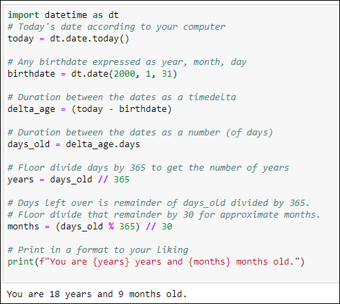
FIGURE 1-18: Calculating age in years and months from a timedelta object.
Accounting for Time Zones
As you know, when it's noon in your neighborhood, it doesn't mean its noon everywhere. Figure 1-19 shows a map of all the time zones. If you want a closer look, simply search the web for time zone map. At any given moment, it’s a different day and time of day depending on where you happen to be on the globe. There is a universal time, called the Coordinated Universal Time or Universal Time Coordinated (UTC). You may have heard of Greenwich Mean Time (GMT) or Zulu time used by the military, which is the same idea. All these times refer to the time at the prime meridian on Earth, or 0 degrees longitude, smack dab in the middle of the time zone map in Figure 1-19.
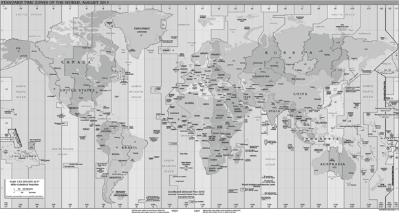
FIGURE 1-19: Time zones.
These days, most people rely on the Olson Database as the primary source of information about time zones. It lists all current time zones and locations. Do a web search for Olson database or tz database if you're interested in all the details. There are too many time zone names to list here, but Table 1-10 shows some examples of American time zones. The left column is the official name from the database. The second column shows the more familiar name. The last two columns show the offset from UTC for standard time and daylight saving time.
TABLE 1-10 Sample Time Zones from the Olson Database
Time Zone |
Common Name |
UTC Offset |
UTC DST Offset |
|---|---|---|---|
Etc/UTC |
UTC |
+00:00 |
+00:00 |
Etc/UTC |
Universal |
+00:00 |
+00:00 |
America/Anchorage |
US/Alaska |
−09:00 |
−08:00 |
America/Adak |
US/Aleutian |
−10:00 |
−09:00 |
America/Phoenix |
US/Arizona |
−07:00 |
−07:00 |
America/Chicago |
US/Central |
−06:00 |
−05:00 |
America/New_York |
US/Eastern |
−05:00 |
−04:00 |
America/Indiana/Indianapolis |
US/East-Indiana |
−05:00 |
−04:00 |
America/Honolulu |
US/Hawaii |
−10:00 |
−10:00 |
America/Indiana/Knox |
US/Indiana-Starke |
−06:00 |
−05:00 |
America/Detroit |
US/Michigan |
−05:00 |
−04:00 |
America/Denver |
US/Mountain |
−07:00 |
−06:00 |
America/Los Angeles |
US/Pacific |
−08:00 |
−07:00 |
Pacific/Pago_Pago |
US/Samoa |
−11:00 |
−11:00 |
Etc/UTC |
UTC |
+00:00 |
+00:00 |
Etc/UTC |
Zulu |
+00:00 |
+00:00 |
So why are we telling you all this? Because Python lets you work with two different types of datetimes:
- Naïve datetime: Any datetime that does not include information that relates it to a specific time zone
- Aware datetime: A datetime that includes time zone information
The timedelta objects and dates that you define with .date() are always naïve. Any time or datetime you create as time() or datetime() objects will also by naïve, by default. But with those two you have the option of including time zone information if it's useful in your work, such as when you're showing event dates to an audience in multiple time zones.
Working with Time Zones
When you get the time from your computer’s system clock, it's for your time zone, but you don't have an indication of what that time zone is. But you can tell the difference between your time and UTC time by comparing .now() for your location to .utc_now() for UTC time, and then subtracting the difference, as shown in Figure 1-20.

FIGURE 1-20: Determining the difference between your time and UTC time.
When we ran that code, the current time was 1:02PM and the UTC time was 6:02PM. The difference was 5:00:00, which means five hours (no minutes or seconds). Our time is earlier, so our time zone is really UTC – 5 hours.
Note that if you subtract the earlier time from the later time, you get a negative number, which can be misleading, as follows:
time_difference = (here_now - utc_now)
Difference: -1 day, 19:00:00
That's still five hours, really, because if you subtract 1 day and 19 hours from 24 hours (one day), you still get 5 hours. Tricky business. But keep in mind the left side of the time zone map is east, and the sun rises in the east in each time zone. So when it’s rising in your time zone, it’s already risen in time zones to the right, and hasn’t yet risen in time zones to your left.
If you want to work directly with time zone names, you’ll need to import some date utilities from Python's dateutils package. In particular, you need gettz (short for get timezone) from the tz class of dateutil. So in your code, right after the line where you import datetime, use from dateutil.tz import gettz like this:
# import datetime and dateutil tz
import datetime as dt
from dateutil.tz import gettz
Afterwards, you can use gettz('name') to get time zone information for any time zone. Replace name with the name of the time zone from the Olson database: for example, America/New_York for USA Eastern Time, or Etc_UTC for UTC Time.
Figure 1-21 shows an example where we get the current date and time using datetime.now() with five different time zones — UTC and four US time zones.
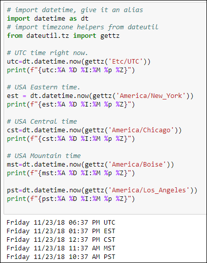
FIGURE 1-21: The current date and time for five different time zones.
All USA times are standard time because no one in the USA is on daylight saving time (DST) in late November. Let's see what happens if we schedule an event for some time in July, when the USA is on back on daylight saving time.
In this code (see Figure 1-22), we import datetime and gettx from dateutil, as we did in the preceding example. But we're not concerned about the current time. We're concerned about an event scheduled for July 4, 2020 at 7:00 PM in our local time zone. So we define that using the following:
event = dt.datetime(2020,7,4,19,0,0)

FIGURE 1-22: Date and time for a scheduled event in multiple time zones.
We didn't say anything about time zone in the date time, so the time will automatically be for our time zone. That datetime is stored in the event variable.
The following line of code (after the comment, which starts with #) shows the date and time, again local, because we didn't say anything about time zone. We added "Local:" to the start of the text, and added a line break at the end (
) to visually separate that word from the rest of the output.
# Show local date and time
print("Local: " + f"{event:%D %I:%M %p %Z}" + "
")
When the app runs, it displays the following output based on the datetime and our format string:
Local: 07/04/20 07:00 PM
The remaining code calculates the correct datetime for each of five time zones:
name = event.astimezone(gettz("tzname"))
The first name is just a variable name we made up. In event.astimezone(), the name event refers to the initial event time defined in a previous line. The astimezone() function is a built-in dateutil function that uses the following syntax:
.astimezone(gettz("tzname"))
In each line of code that calculates the date and time for a time zone, we replace tzname with the name of the time zone from the Olson database. As you can see in the output (refer to Figure 1-22), the datetime of the event for five different time zones is displayed. Note that the USA time zones are daylight saving time (such as EDT). Because we happen to be on the east coast and the event is in July, the correct local time zone is Eastern Daylight Time. When you look at the output of the dates, the first one matches our time zone, as it should, and the times for the remaining dates are adjusted for different time zones.
If you're thinking “Eek, what a complicated mess,” you won't get any argument from us. None of this strikes us as intuitive, easy, or in the general ballpark of fun. But if you're in a pinch and need some time zone information for your data, the coding techniques you've learned so far should get you want you need.
If you research Python time zones online, you’ll probably find that many people recommend using the arrow module rather than the dateutil module. We won't get into all that here, because arrow isn’t part of your initial Python installation and this book is hefty enough. (If we tried to cover everything, you’d need a wheelbarrow to carry the book around.)