
Chapter 3
Using Big Data from Google Cloud
IN THIS CHAPTER
![]() Accessing really big data
Accessing really big data
![]() Using Google Cloud BigQuery
Using Google Cloud BigQuery
![]() Building your first queries
Building your first queries
![]() Visualizing results with MatPlotLib
Visualizing results with MatPlotLib
Up to this point, you've been dealing with relatively small sets of data. In this chapter, you use big data from the Medicare database and then very big data from NOAA (National Oceanic and Atmospheric Agency) that changes every hour!
Even if you have access to a powerful enough computer to download large datasets like these, not every big dataset can be downloaded. Some datasets can't be downloaded legally. And in the case of the air quality database from NOAA, you would have to download a new version every hour. In cases like these, it’s better to leave the data where it is and use the cloud. In addition, when you let the cloud do the database and analysis work, your computer doesn’t have to be very big or very fast.
To download the code for this chapter, go to www.dummies.com/go/pythonaiofd2e.
What Is Big Data?
Big data refers to datasets that are too large or complex to be dealt with using traditional data-processing techniques. Data with many cases and many rows offers greater accessibility to sophisticated statistical techniques and generally lead to smaller false discovery rates. A false discovery rate is the expected proportion of errors where you incorrectly rejected your hypothesis (in other words, you received false positives).
As mentioned in Chapter 1 of this minibook, big data is becoming more prevalent in our society as the number of computers and sensors proliferate and create more data at an ever-increasing rate. In this chapter, we talk about using the cloud to access these large databases (using Python and Pandas) and then visualizing the results on a Raspberry Pi.
Understanding Google Cloud and BigQuery
In the first program, you access data using Google Cloud and manipulate and analyze the data using Google BigQuery. It is important to understand that you aren’t just using data in the cloud, you're also using the data analysis tools in the cloud. Basically, you're using your computer to tell the computers in the cloud what do with the data and how to analyze it. Not much is happening on your local computer.
Google Cloud Platform
Google Cloud Platform is a suite of cloud-computing services that run on the same infrastructure as Google end-user products such as Google Search and YouTube. This cloud strategy has been successfully used at Amazon and Microsoft. Google uses their own internal data services and products to build a cloud offering. With this approach, both the user and the company benefit from advances and improvements to products and clouds.
The Google Cloud Platform has over 100 different APIs (application programming interfaces) and data service products available for data science and artificial intelligence. The primary service we use in this chapter is the Google API called BigQuery.
BigQuery from Google
A REST (representational state transfer) software system defines a set of communication structures to be used for creating web services, typically using http and https requests to communicate. With a REST-based system, different computers and different operating systems can enable the same web service.
A RESTful web service uses URL addresses that ask specific questions in a standard format and get a response just like a browser gets a web page. Additional Python libraries are used to hide the complexity of the queries going back and forth. BigQuery is based on a RESTful web service.
In software engineering, abstraction is a technique for arranging complexity in computer systems. It works by establishing a simple layer in the software (such as Python modules) that masks the complex details below the surface. Abstraction in software systems is key to making big systems work and reasonable to program. For example, although a web browser uses HTML to display web pages, layers of software under the HTML are doing such things such as transmitting IP packets or manipulating bits. These lower layers are different if you're using a wired network or a Wi-Fi network. The cool thing about abstraction is that we don’t need to know how complex it is. We just use the software.
BigQuery is a serverless model, which means BigQuery has one of the highest levels of abstraction in the cloud community, removing the user’s responsibility for bringing new virtual machines online, the amount RAM, the numbers of CPUs, and so on. Scale from one to thousands of CPUs in a matter of seconds, paying only for the resources you use. You can stream data into BigQuery on the order of millions of rows (data samples) per second, which means you can start to analyze the data almost immediately. Google Cloud has a free, 90-day trial with $300 of credit, so you won’t have to pay while working on the examples in Book 5.
BigQuery has a large number of public big-data datasets; we access the ones from Medicare and NOAA. We use BigQuery (through the google.cloud library) with the Pandas Python library. The google.cloud Python library maps the BigQuery data into our friendly Pandas DataFrames (described in Chapter 2 of this minibook).
Computer security on the cloud
We would be remiss if we didn’t talk just a little bit about maintaining good computer security when using the cloud. Google provides computer security by using the IAM (identity and access management) paradigm throughout its cloud offerings. IAM lets the account owner (who is the administrator) authorize who can take what kind of action on specific resources, giving the owner full control and visibility for simple projects as well as finely grained access extending across an entire enterprise.
We show you how to set up IAM authentication in the sections that follow.
Signing up for BigQuery
Go to https://cloud.google.com and sign up for your free trial. Although Google requires a credit card to prove that you're not a robot, it doesn't charge you even when your trial is over unless you manually switch to a paid account. If you exceed $300 during your trial (which you probably won’t), Google will notify you but will not charge you. The $300 limit should be more than enough to do a bunch of queries and learn on the BigQuery cloud platform.
Reading the Medicare Big Data
In this section, to start using BigQuery with your own Python programs, you set up a project and download your authentication .json file, which contains keys that let you access your account and the data. The Medicare database is the largest easily accessible medical data set in the world. We ask some specific medical queries of this database.
Setting up your project and authentication
To access Google Cloud, you need to set up a project and then receive your authentication credentials from Google.
 Make sure you follow these directions closely to get the Google authentication correct the first time. When you download your authentication file, don’t lose it or delete it. You can’t download it a second time. Instead, you have to go through the authentication process again.
If you don’t have a Google account, create one. Then go to www.google.com and log in,. Next, go to https://developers.google.com/ and click Google Cloud. Fill out your billing information, and you'll be ready to begin.
The following steps will show you how to set up your project and get your authentication credentials:
Go to
https://console.developers.google.com/and sign in using your account name and password.The screen shown in Figure 3-1 appears.
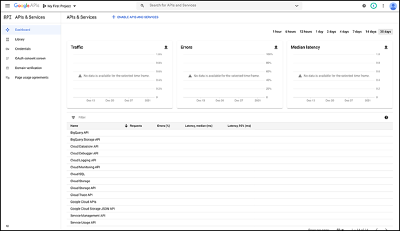
FIGURE 3-1: Google Cloud developer's console page.
- Click the My First Project button, in the upper-left corner of the screen.
- On the pop-up screen, click the New Project button in the upper right.
For the project name, type MedicareProject and then click Create.
You return to the screen shown in Figure 3-1.
In the drop-down menu on the upper left, choose MedicareProject.
 Make sure you change the selection to MedicareProject and don't leave the default as My First Project. Otherwise, you'll be setting up the APIs and authentication for the wrong project. This mistake is a very common one.
Click the +Enable APIs and Services button (near the top) to enable the BigQuery API.
The API selection screen appears.
In the search box, search for BigQuery and then select BigQuery API. Click Enable.
Now to get our authentication credentials.
In the right corner of the screen, choose Create Credentials.
The screen shown in Figure 3-2 appears.
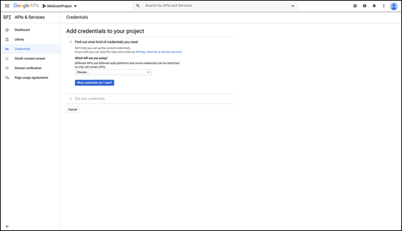
FIGURE 3-2: First credentials screen.
- In the drop-down menu, select BigQuery API and then click the No, I'm Not Using Them option below the Are You Planning to Use This API with the App Engine or Compute Engine? section.
Click the What Credentials Do I Need? button.
The screen shown in Figure 3-3 appears.
- In the Service Account Name box, type MedicareProject and then, in the Role drop-down menu, select Project and then select Owner.
Leave the JSON radio button selected and click Continue.
A message appears saying that the service account and key have been created. A file named something like
MedicareProject-1223xxxxx413.jsonis downloaded to your computer. Do not lose this file! It contains your authentication information.- Copy the downloaded file to the directory where you'll be building your Python program file.
Now let’s move on to our first example.

FIGURE 3-3: Second credentials screen.
The first big-data code
The MedicareQuery1.py program reads one of the several dozen public-data Medicare datasets and grabs some data for analysis. We will use the inpatient_charges_2015 dataset and a SQL query to select the information from the dataset that we want to look at and analyze. (Check out the nearby sidebar, “Learning SQL,” for more on SQL if you're not already familiar with this ubiquitous query language.)
Table 3-1 shows all the columns in the inpatient_charges_2015 dataset.
TABLE 3-1 Columns, Types, and Descriptions of the inpatient_charges_2015 Dataset
Column |
Type |
Description |
|---|---|---|
|
STRING |
The CMS certification number (CCN) of the provider billing for outpatient hospital services. |
|
STRING |
The name of the provider. |
|
STRING |
The street address in which the provider is physically located. |
|
STRING |
The city in which the provider is physically located. |
|
STRING |
The state in which the provider is physically located. |
|
INTEGER |
The zip code in which the provider is physically located. |
|
STRING |
The code and description identifying the MS-DRG. MS-DRGs are a classification system that groups similar clinical conditions (diagnoses) and the procedures furnished by the hospital during the stay. |
|
STRING |
The hospital referral region (HRR) in which the provider is physically located. |
|
INTEGER |
The number of discharges billed by the provider for inpatient hospital services. |
|
FLOAT |
The provider's average charge for services covered by Medicare for all discharges in the MS-DRG. These vary from hospital to hospital because of differences in hospital charge structures. |
|
FLOAT |
The average total payments to all providers for the MS-DRG, including the MS-DRG amount, teaching, disproportionate share, capital, and outlier payments for all cases. Also included in average total payments are co-payment and deductible amounts that the patient is responsible for and any additional third-party payments for coordination of benefits. |
|
FLOAT |
The average amount that Medicare pays to the provider for its share of the MS-DRG. Average Medicare payment amounts include the MS-DRG amount, teaching, disproportionate share, capital, and outlier payments for all cases. Medicare payments do not include beneficiary co-payments and deductible amounts nor any additional payments from third parties for coordination of benefits. |
Using nano (or another text editor), enter the following code and then save it as MedicareQuery1.py:
import pandas as pd
from google.cloud import bigquery


# set up the query

QUERY = """
        SELECT provider_city, provider_state, drg_definition,
        average_total_payments, average_medicare_payments
        FROM `bigquery-public-data.cms:medicare.inpatient_charges_2015`
        WHERE provider_city = "GREAT FALLS" AND provider_state = "MT"
        ORDER BY provider_city ASC
        LIMIT 1000
        """

client = bigquery.Client.from:service_account_json(
            'MedicareProject2-122xxxxxf413.json')


query_job = client.query(QUERY)
df = query_job.to_dataframe()

print ("Records Returned: ", df.shape )
print ()
print ("First 3 Records")
print (df.head(3))
As soon as you've built this file, replace the MedicareProject2-122xxxxxf413.json file with your own authentication file (which you copied into the program directory earlier).
 When you run the
 MedicareQuery1.py program, you'll get an import error if the google.cloud library isn't installed. If this happens, type the following in the Terminal window on your computer:
sudo pip3 install google-cloud-bigquery
When running these programs on a Raspberry Pi, if you see an error that “the pyarrow library is not installed,” try the following:
sudo pip3 install pyarrow
As of November 2020, if installing pyarrow doesn't work, the pyarrow maintainers have not yet fixed the problem with the pip3 pyarrow installation. You will need to move to Windows, another Linux version, or a Mac to run these examples.
Breaking down the code
First, we import our libraries. Note the google.cloud library and the bigquery import:
import pandas as pd
from google.cloud import bigquery
Next we set up a SQL query to fetch the data into a Pandas DataFrame for analysis:
# set up the query

QUERY = """
        SELECT provider_city, provider_state, drg_definition,
        average_total_payments, average_medicare_payments
        FROM `bigquery-public-data.cms:medicare.inpatient_charges_2015`
        WHERE provider_city = "GREAT FALLS" AND provider_state = "MT"
        ORDER BY provider_city ASC
        LIMIT 1000
        """
See the structure of the SQL query? We SELECT the columns that we want (as listed in Table 3-1) FROM the bigquery-public-data.cms:medicare.inpatient_charges_2015 database only WHERE the provider_city is GREAT FALLS and the provider_state is MT. Finally, we tell the system to order the results by ascending, alphanumeric order by the provider_city.
Remember to replace the following json filename with your authentication file:
client = bigquery.Client.from:service_account_json(
            'MedicareProject2-122xxxxxef413.json')
Now we fire off the query to BigQuery:
query_job = client.query(QUERY)
And translate the results to our good friend the Pandas DataFrame:
df = query_job.to_dataframe()
Now just a few more code statements to display what we get back from BigQuery:
print ("Records Returned: ", df.shape )
print ()
print ("First 3 Records")
print (df.head(3))
Run your program MedicareQuery1.py and you should see the results of your query as shown next. If you get an authentication error, make sure you put the correct authentication file into your directory. And if necessary, generate another authentication file, paying special attention to the project name selection.
Records Returned:  (112, 5)

First 3 Records
  provider_city provider_state
drg_ definition  average_total_payments  average_medicare_payments
0   GREAT FALLS             MT  064 - INTRACRANIAL HEMORRHAGE OR CEREBRAL INFA…                11997.11                   11080.32
1   GREAT FALLS             MT           039 - EXTRACRANIAL PROCEDURES W/O
CC/MCC                 7082.85                    5954.81
2   GREAT FALLS             MT  065 - INTRACRANIAL HEMORRHAGE OR CEREBRAL
INFA…                 7140.80                    6145.38
Visualizing your Data
We found 112 records from Great Falls. You can go back and change the query in your program to select your own city and state.
Doing a bit of analysis
You've established a connection to a big-data database. Now let's set up another query. We will search the entire inpatient_charges_2015 dataset to look for patients with MS_DRG code 554, bone diseases and arthropathies without major complication or comorbidity (in other words, people who have issues with their bones but with no serious issues currently manifesting externally). We find such a diagnosis through one of the most arcane and complicated coding systems in the world: ICD-10, which maps virtually any diagnostic condition to a single code.
Create a file called MedicareQuery2.py using nano or your favorite text editor, and then copy the following code into the file:
import pandas as pd
from google.cloud import bigquery


# set up the query

QUERY = """
        SELECT provider_city, provider_state, drg_definition,
        average_total_payments, average_medicare_payments
        FROM `bigquery-public-data.cms:medicare.inpatient_charges_2015`
        WHERE drg_definition LIKE  '554 %'
        ORDER BY provider_city ASC
        LIMIT 1000
        """

client = bigquery.Client.from:service_account_json(
            'MedicareProject2-1223283ef413.json')


query_job = client.query(QUERY)
df = query_job.to_dataframe()

print ("Records Returned: ", df.shape )
print ()
print ("First 3 Records")
print (df.head(3))
The only thing different in this program from our previous one is that we added LIKE '554 %', which matches any DRG that starts with 554.
When we ran the program, we got the following results:
Records Returned:  (286, 5)

First 3 Records
  provider_city provider_state                               drg_definition  average_total_payments  average_medicare_payments
0      ABINGTON             PA  554 - BONE DISEASES & ARTHROPATHIES W/O MCC                 5443.67                    3992.93
1         AKRON             OH  554 - BONE DISEASES & ARTHROPATHIES W/O MCC                 5581.00                    4292.47
2        ALBANY             NY  554 - BONE DISEASES & ARTHROPATHIES W/O MCC                 7628.94                    5137.31
Now we have some interesting data. Let’s do a little analysis. What percent of the total payments for this condition is paid by Medicare? The remainder is usually paid by the patient. We aren’t taking third-party billing into account.
Create a file called MedicareQuery3.py using nano or your favorite text editor, and copy the following code into the file:
import pandas as pd
from google.cloud import bigquery


# set up the query

QUERY = """
        SELECT provider_city, provider_state, drg_definition,
        average_total_payments, average_medicare_payments
        FROM `bigquery-public-data.cms:medicare.inpatient_charges_2015`
        WHERE drg_definition LIKE  '554 %'
        ORDER BY provider_city ASC
        LIMIT 1000
        """

client = bigquery.Client.from:service_account_json(
            'MedicareProject2-1223283ef413.json')


query_job = client.query(QUERY)
df = query_job.to_dataframe()

print ("Records Returned: ", df.shape )
print ()

total_payment = df.average_total_payments.sum()
medicare_payment = df.average_medicare_payments.sum()

percent_paid = ((medicare_payment/total_payment))*100
print ("Medicare pays {:4.2f}% of Total for 554 DRG".format(percent_paid))
print ("Patient pays {:4.2f}% of Total for 554 DRG".format(100-percent_paid))
The results follow:
Records Returned: (286, 5)
Medicare pays 77.06% of Total for 554 DRG
Patient pays 22.94% of Total for 554 DRG
Payment percent by state
Next, we select each individual state in our database (not all states are represented) and calculate the percent paid by Medicare by state for a DRG that starts with 554. Call this file MedicareQuery4.py:
import pandas as pd
from google.cloud import bigquery


# set up the query

QUERY = """
        SELECT provider_city, provider_state, drg_definition,
        average_total_payments, average_medicare_payments
        FROM `bigquery-public-data.cms:medicare.inpatient_charges_2015`
        WHERE drg_definition LIKE  '554 %'
        ORDER BY provider_city ASC
        LIMIT 1000
        """

client = bigquery.Client.from:service_account_json(
            'MedicareProject2-1223283ef413.json')


query_job = client.query(QUERY)
df = query_job.to_dataframe()

print ("Records Returned: ", df.shape )
print ()

# find the unique state values

states = df.provider_state.unique()
states.sort()

total_payment = df.average_total_payments.sum()
medicare_payment = df.average_medicare_payments.sum()

percent_paid = ((medicare_payment/total_payment))*100
print("Overall:")
print ("Medicare pays {:4.2f}% of Total for 554 DRG".format(percent_paid))
print ("Patient pays {:4.2f}% of Total for 554 DRG".format(100-percent_paid))

print ("Per State:")

# now iterate over states

print(df.head(5))
state_percent = []
for current_state in states:
    state_df = df[df.provider_state == current_state]

    state_total_payment = state_df.average_total_payments.sum()

    state_medicare_payment = state_df.average_medicare_payments.sum()

    state_percent_paid = ((state_medicare_payment/state_total_payment))*100
    state_percent.append(state_percent_paid)

    print ("{:s} Medicare pays {:4.2f}% of Total for 554 DRG".format
 (current_state,state_percent_paid))
Now some visualization
For our last experiment, we use MatPlotLib to visualize the state-by-state data in a graph generated by the MedicareQuery4.py program.
Do you already have seaborn on your Raspberry Pi? (If you've installed MatPlotLib, you probably do.) To find out, run the MedicareQuery4.py example Python program. If seaborn isn't installed, you'll see import errors and should then run the following command:
sudo apt-get install python3-seaborn
Moving to our VNC program so we can have a GUI on our Raspberry Pi, add the following code to the end of the preceding MedicareQuery4.py code:
# We could graph this using MatPlotLib with the two lists,
# but we want to use DataFrames for this example

data_array = {'State': states, 'Percent': state_percent}

df_states = pd.DataFrame.from:dict(data_array)

# Now back in dataframe land
import matplotlib.pyplot as plt
import seaborn as sb

print (df_states)

df_states.plot(kind='bar', x='State', y= 'Percent')
plt.show()
Figure 3-4 shows the resulting graph from running the MedicareQuery4.py program.
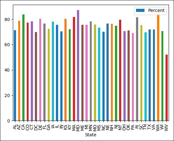
FIGURE 3-4: Bar chart of Medicare percent paid per state for code 554.
Looking for the Most Polluted City in the World on an Hourly Basis
Just one more quick example. Another public database on BigQuery called OpenAQ contains air-quality measurements from 47 countries around the world. And this database is updated hourly, believe it or not.
Here is some code that picks up the top three worst polluted cities in the world, as measured by air quality:
import pandas as pd
from google.cloud import bigquery

# sample query from:
QUERY = """
        SELECT location, city, country, value, timestamp
        FROM `bigquery-public-data.openaq.global_air_quality`
        WHERE pollutant = "pm10" AND timestamp > "2017-04-01"
        ORDER BY value DESC
        LIMIT 1000
        """

client = bigquery.Client.from:service_account_json(
                    'MedicareProject2-1223283ef413.json')
query_job = client.query(QUERY)
df = query_job.to_dataframe()

print (df.head(3))
Copy this code into a file called PollutedCity.py and run the program. Following is the current result of running the code (as of this writing):
        location          city country  value    timestamp
0       Dilovası        Kocaeli   TR  5243.00 2018-01-25 12:00:00+00:00
1  Bukhiin urguu    Ulaanbaatar   MN  1428.00 2019-01-21 17:00:00+00:00
2  Chaiten Norte  Chaiten Norte   CL   999.83 2018-04-24 11:00:00+00:00
Dilovasi, Kocaeli, Turkey is not a healthy place to be right now. Doing a quick Google search of Dilovasi finds that cancer rates are three times higher than the worldwide average. This striking difference apparently stems from the environmental heavy metal pollution that has persisted in the area for about 40 years, mainly due to intense industrialization.
John will definitely be checking this on a daily basis.