In this chapter, you will learn how to create, translate, and rotate three-dimensional objects in a three-dimensional space. You will also learn how to project and display them on the two-dimensional surface of your computer screen. General movement of an object implies both translation and rotation. I discussed this in two dimensions in the previous chapter. You saw that translation in two dimensions is trivial. Just add or subtract a quantity from the x coordinates to translate in the x direction, similarly for the y direction. In three dimensions, it is still trivial, although you are able now to translate in the third dimension, the z direction, simply by adding or subtracting an amount to an object’s z coordinates. Rotation is another matter, however. The analysis follows the method you used in two dimensions but is complicated by the fact that you now are able to rotate an object around three coordinate directions. In this chapter, I will not discuss 3D translation any further but will concentrate instead on 3D rotation.
3.1 The Three-Dimensional Coordinate System

Three-dimensional coordinate axes with point P at coordinates (x,y,z)
It should be apparent now why I used the nomenclature Rz in the previous discussion of two-dimensional rotation; it refers to rotation about the z axis. This appears as a clockwise rotation in the x-y plane when x goes to the right and y goes down. If x went to the right and y were to go up, z would point out of the screen and a positive rotation about the z axis would appear to go counterclockwise.
Following the methods used in this analysis of two-dimensional rotation, in the remainder of this chapter I will discuss separate rotations around the x,y, and z axes and then combined rotations around all three axes. Incidentally, when I say “rotation around the x axis”, for example, I am implying that this is equivalent to “rotation around the x direction” and vice versa. While rotation around an imaginary axis that is parallel to the x axis is not precisely the same as rotation around the x axis, the difference is only a matter of translation. I will use both terms interchangeably except when confusion may result.
Figure 3-2 shows the right-hand x,y,z system . Imagine you’re standing at the origin, looking out in the direction of the x axis. If you were to turn a right-handed screw clockwise, it would progress in the direction of the positive x axis. The double-headed arrow is the conventional way of indicating the direction of a right-hand rotation, Rx; similarly for Ry and Rz.
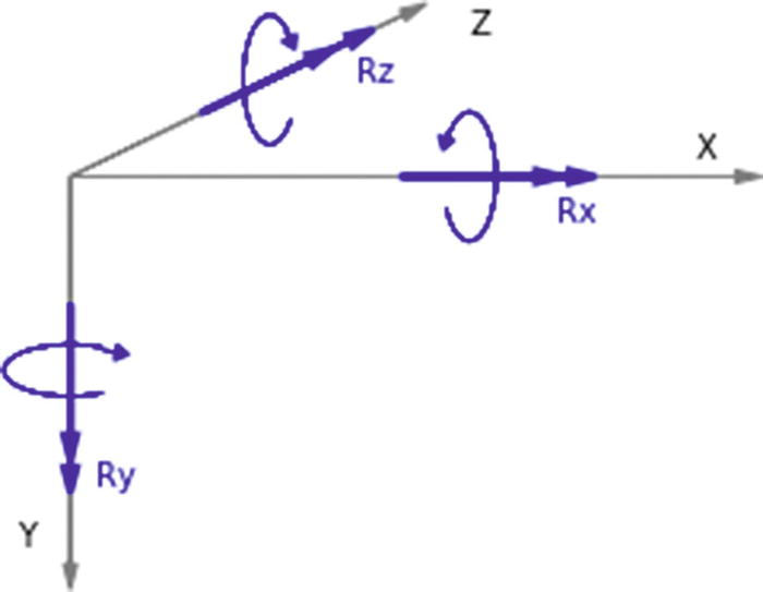
Three-dimensional coordinate axes showing right-hand rotation around each coordinate direction
As explained earlier, the orientation in Figure 3-2 is somewhat more intuitive. The object being constructed is inside a space defined by the x,y,z axes. In this situation, the observer is outside the space looking in. The object may be translated and rotated at will to give any view desired. You can look straight in at an object or view it from above or below, as shown in the images of Saturn in Chapter 10. The matplotlib orientation, on the other hand, is the one commonly used for data plotting and is the one you’ll use for that purpose in Chapter 9; look at Figures 9-1 through 9-5. If you prefer the standard matplotlib system, it is easy to change to that orientation; just rotate the axes to any orientation you want, as is done in Chapter 9 where, to get z pointing up, you rotate around the global x direction by -100 degrees (tilts z slightly forward), the global y axis by -135 degrees, and the global z direction by +8 degrees (see lines 191-193 in Listing 9-1). You can fine-tune the orientation by small rotations about the global axes. After you complete this chapter, you should find it easy to shade the background planes, as shown in matplotlib, if you want. You can orient the axes any way you want as long as they follow the right-hand rule.
3.2 Projections onto the Coordinate Planes

Projection of a three-dimensional line (black) onto the three coordinate planes: red=x,z projection, green=y,z projection, and blue=x,y projection
The x,y projection is obtained by plotting a point’s x and y coordinates in the x,y plane; for a line, you plot a line between the x and y coordinates of the line’s endpoints. In the case of the black line, which runs from spatial coordinates (xA,yA,zA) to (xB,yB,zB), you plot a line between xA,yA and xB,yB:
This gives you the blue line, which is the projection onto the x,y plane as shown in Figure 3-4. If you want to obtain the top view, you plot the black line’s z,x coordinates. If plotting with your normal coordinate axes with x running from left to right and y running down on the left, the y axis replaces the z axis. This is equivalent to a -90 degree rotation about the x axis. You then plot between the line’s z and x coordinates of
to get the red line. To get the green y, z projection, you plot the z and y coordinates using the command

Projection of a three-dimensional line onto the x, y plane
In this case, you must reorient the screen coordinate axes such that +z runs from left to right across the top of the screen with the y axis running down the right side. This will give a z, y view from outside of the x,y,z coordinate system.
Note that in the case of a projection onto the x,y plane, you do not use the object’s z coordinates. But you still need them in order to carry out rotations. Similarly for the other projections, one coordinate is not needed for the projection but is needed for rotations so it must be included in the analysis.
To simplify everything, you will use the x,y projection in most of the work that follows. As you will see, rotating an object around the three coordinate directions and projecting the object’s (x,y) coordinates onto the x,y plane will produce a three-dimensional view.
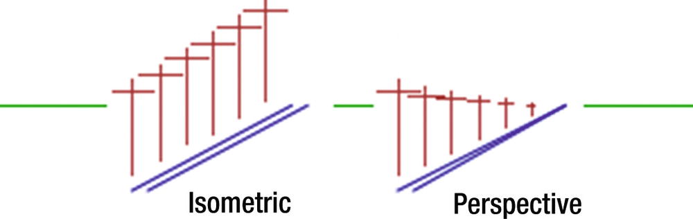
Isometric vs. perspective views
While you have seen how to project a simple three-dimensional line and its end points onto the three coordinate planes, you could have worked with a more complicated object consisting of many points and lines . As you have seen, even a circle can be constructed from just points (dots) or lines with any degree of refinement desired.
While a simple example, the three-dimensional line illustrates the method you will use in the following work: define a shape within the three-dimensional x,y,z space in terms of points and lines having coordinates (x,y,z); operate on them by rotating and translating; project them onto the x,y plane; and then plot them using their x and y coordinates. Thus you are able to project a 3D object onto your computer monitor’s screen.
To rotate a point in three dimensions implies rotating it around the x,y, and z directions. You saw how to carry out two-dimensional rotation around the z direction, Rz, in the previous chapter. Here, you will derive transformations in three dimensions for rotation around the y,x, and z directions.
3.3 Rotation Around the y Direction
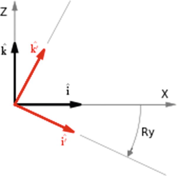
Unit vectors for rotation about the y direction. This is a view looking down on the plotting space. The y axis runs into the plane of the paper.


![$$ {mathbf{P}}^{prime }= xpleft[mathit{cos}(Ry)widehat{mathbf{i}}-mathit{sin}(Ry)widehat{mathbf{k}}
ight]+ ypwidehat{mathbf{j}}+ zpleft[mathit{sin}(Ry)widehat{mathbf{i}}+mathit{cos}(Ry)widehat{mathbf{k}}
ight] $$](http://images-20200215.ebookreading.net/10/3/3/9781484233788/9781484233788__python-graphics-a__9781484233788__images__456962_1_En_3_Chapter__456962_1_En_3_Chapter_TeX_Equ7.png)
![$$ {mathbf{P}}^{prime }=underset{x{p}^{prime }}{underbrace{left[ xpcos(Ry)+ zpkern0.1em mathit{sin}(Ry)
ight]}}widehat{mathbf{i}}+underset{y{p}^{prime }}{underbrace{left[ yp
ight]}}widehat{mathbf{j}}+underset{z{p}^{prime }}{underbrace{left[- xpkern0.1em mathit{sin}(Ry)+ zpkern0.1em mathit{cos}(Ry)
ight]}}widehat{mathbf{k}} $$](http://images-20200215.ebookreading.net/10/3/3/9781484233788/9781484233788__python-graphics-a__9781484233788__images__456962_1_En_3_Chapter__456962_1_En_3_Chapter_TeX_Equ8.png)


Equations 3-9 through 3-11 give the coordinates of the rotated point in the local x,y,z system. Of course, yp′=yp in Equation 3-10 since the y coordinate doesn’t change with rotation about the y axis.

![$$ left[{P}^{hbox{'}}
ight]=left[ Ry
ight]kern0.1em left[P
ight] $$](http://images-20200215.ebookreading.net/10/3/3/9781484233788/9781484233788__python-graphics-a__9781484233788__images__456962_1_En_3_Chapter__456962_1_En_3_Chapter_TeX_Equ13.png)


These elements will be used in the programs that follow.
3.4 Rotation Around the x Direction
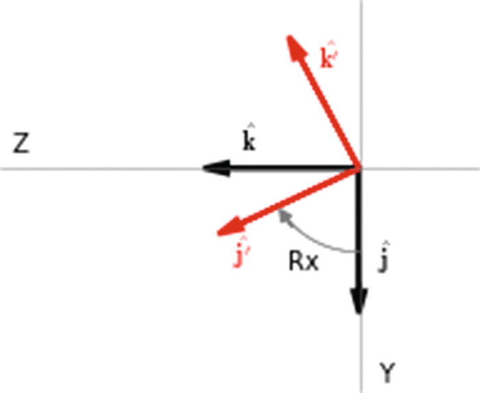
Unit vectors for rotation around the x direction. The x axis runs into the plane of the paper.


![$$ {mathbf{P}}^{prime }= xpwidehat{mathbf{i}}+ ypleft[mathit{cos}(Rx)widehat{mathbf{j}}+mathit{sin}(Rx)widehat{mathbf{k}}
ight]+ zpleft[-mathit{sin}(Rx)widehat{mathbf{j}}+mathit{cos}(Rx)widehat{mathbf{k}}
ight] $$](http://images-20200215.ebookreading.net/10/3/3/9781484233788/9781484233788__python-graphics-a__9781484233788__images__456962_1_En_3_Chapter__456962_1_En_3_Chapter_TeX_Equ28.png)
![$$ =underset{x{p}^{prime }}{underbrace{xp}}widehat{mathbf{i}}+underset{y{p}^{prime }}{underbrace{left[ ypkern0.1em mathit{cos}(Rx)- zpkern0.1em mathit{sin}(Rx)
ight]}}widehat{mathbf{j}}+underset{z{p}^{prime }}{underbrace{left[ ypkern0.1em mathit{sin}(Rx)+ zpkern0.1em mathit{cos}(Rx)
ight]}}widehat{mathbf{k}} $$](http://images-20200215.ebookreading.net/10/3/3/9781484233788/9781484233788__python-graphics-a__9781484233788__images__456962_1_En_3_Chapter__456962_1_En_3_Chapter_TeX_Equ29.png)

![$$ left[{P}^{hbox{'}}
ight]=left[ Rx
ight]kern0.1em left[P
ight] $$](http://images-20200215.ebookreading.net/10/3/3/9781484233788/9781484233788__python-graphics-a__9781484233788__images__456962_1_En_3_Chapter__456962_1_En_3_Chapter_TeX_Equ31.png)


3.5 Rotation Around the z Direction


You can extend the two-dimensional matrix equation to three-dimensions in Equation 3-44 by simply observing that in the first row xp′ does not depend on zp, hence C(1,3)=0; in the second row, yp′ also does not depend on zp, hence c(2,3)=0; in the third row, zp′ does not depend on either xp′ or yp′, hence C(3,1) and C(3,2) both equal 0. C(3,3)=1 since the z coordinate remains unchanged after rotation about the z axis.


3.6 Separate Rotations Around the Coordinate Directions

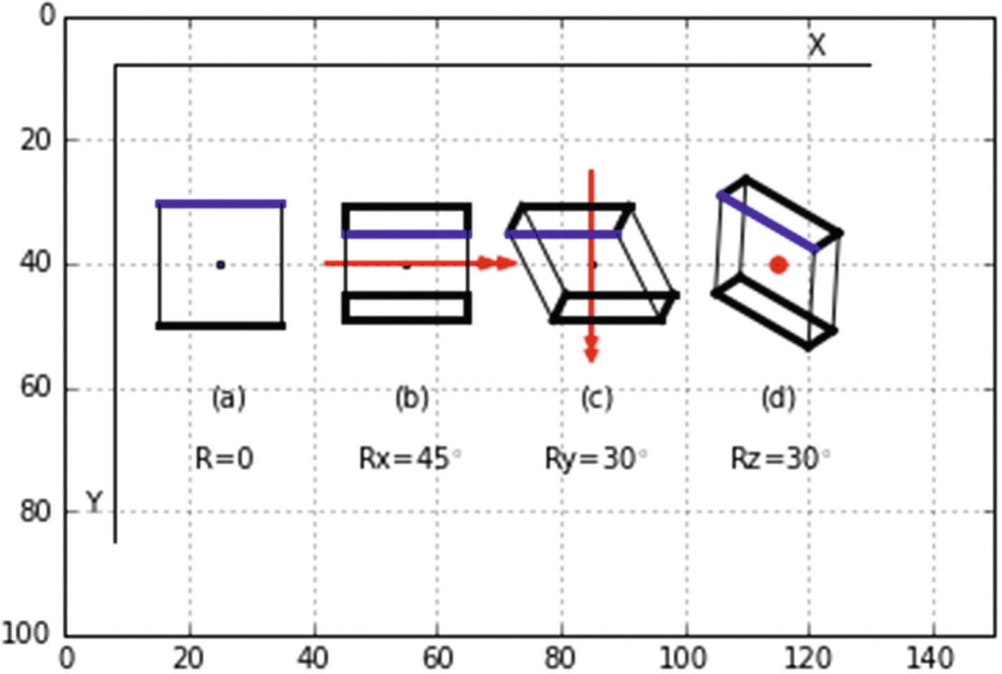
Output from Listing 3-1. Projection (a) of an unrotated box on the x,y plane, (b) rotated around the x direction by Rx=45°, (c) around the y direction by Ry=30°, and (d) around the z direction by Rz=30°. Double-headed red arrows show the direction of rotation using the right-hand rule convention. Heavy lines indicate the top and bottom. The boxes are rotated about their center, which is indicated by a black dot.
Listing 3-1 makes use of functions and lists. Without them, the program would more than double in size. Using them reduces the program size considerably. It could be shortened even further by the use of arrays but the savings would be minimal and tends to obscure the methodology.
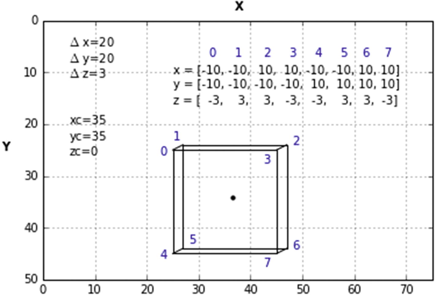
The lists shown in the figure define the corner coordinates . There are eight elements in each list because there are eight corners in the box. Corner 2, which is the third element in the list, has coordinates x[3]=10,y[3]=-10,z[3]=3. These are local coordinates; in other words, they are relative to the box’s center, which is the center of rotation.
Listing 3-1 starts off by defining lists for [x],[y], and [z] in lines 14-16. These lines hold the coordinates of the box’s corners relative to its center. [xg],[yg], and [zg] in lines 18-20 will hold the global plotting coordinates after transformations have been done. Space is reserved for eight in each list since there are eight corners in the box.
Next are the definitions of the rotation functions rotx, roty, and rotz. They rotate a point’s coordinates xp,yp,zp around the x,y, and z directions, respectively. Each function returns a new set of coordinates: xg,yg, and zg, which are the global coordinates of the rotated point. These coordinates will be used for plotting.
Looking at the definition of rotx , which begins in line 23, when invoked to do a transformation about the x direction rotx receives the box’s center coordinates xc,yc,zc, which, in this case is the center of rotation, plus the point’s unrotated coordinates xp,yp,zp and the angle of rotation about the x direction, Rx. The list a=[xp,yp,zp] in line 24 contains the coordinates of the unrotated point. This is, in effect, a vector to point xp,yp,zp. In line 25, b=[1,0,0] is a list of the first row of the Rx transformation matrix shown in Equation 3-55. Line 26, xpp=np.inner(a,b), forms the dot or scalar product of these lists. There is also an np.dot(a,b) function that could be used. For simple non-complex vectors, np.inner(a,b) and np.dot(a,b) give the same results. But for higher dimensional arrays the results may differ.

![$$ a=left[ xp, yp, zp
ight] $$](http://images-20200215.ebookreading.net/10/3/3/9781484233788/9781484233788__python-graphics-a__9781484233788__images__456962_1_En_3_Chapter__456962_1_En_3_Chapter_TeX_Equ59.png)
![$$ b=left[0,mathit{cos}(Rx),-mathit{sin}(Rx)
ight] $$](http://images-20200215.ebookreading.net/10/3/3/9781484233788/9781484233788__python-graphics-a__9781484233788__images__456962_1_En_3_Chapter__456962_1_En_3_Chapter_TeX_Equ60.png)


Next is the function plotbox in line 56. This plots the box using its global corner coordinates xg,yg, and zg. The loop starting in line 57 plots the top by connecting the first three corners with lines. Line 60 closes the top by plotting a line between corners 3 and 0. This has not been included in the loop, which was set up to plot one corner with the next. The problem comes when you try to connect corner 3 with 0; the algorithm in the loop doesn’t work. It could be modified to handle it, but it’s easier to just add line 60 rather than complicate the loop. The rest of plotbox up to line 68 completes the box. Line 70 plots a dot at its center.
Line 72 starts function plotboxx. This transforms the corner coordinates to get them ready for plotting by plotbox. The loop from line 73 to 74 rotates all eight corners around the x direction by invoking rotx. Line 76 invokes function plotbox, which does the plotting. plotboxy and plotboxz do the same for rotations about the y and z directions.
Up to this point, you have been defining functions. You use functions in this program since many of the operations are repetitive. If you tried to write this program using single statements, it would be at least twice as long.
Control of the program lies between lines 91 and 116. Lines 91-95 plot the first box (a). Since this first box (a) is unrotated, you specify Rx=0 in line 91. You use function plotboxx with the Rx=0 parameter to do the plotting. You could use Ry=0 with plotboxy or Rz=0 with plotboxz. It doesn’t matter since the angle of rotation is 0. Lines 92-94 specify the box’s center coordinates. Line 95 invokes plotboxx. The result is shown in Figure 3-8 as (a). Lines 98-116 produce the rotated boxes (b), (c), and (d).
To summarize the procedure using box (b) as an example, the angle of rotation is set in line 98; the box’s center coordinates in lines 99-101. Then, in line 102, function plotboxx is invoked. The center coordinates and the angle Rx are passed as arguments. plotboxx, which begins in line 72, rotates the eight corners by invoking rotx. plotboxx doesn’t use xc,yc, and zc, but it passes them onto rotx, which needs them. rotx rotates and translates the coordinates producing xg,yg,zg. Line 76 invokes function plotbox , which does the plotting.
In lines 91, 98, 105, and 112 you use the function radians(), which was imported from the math library in line 7. (Note that you could have used numpy for this). It converts an argument in degrees to one in radians, which are required by sin() and cos(). In earlier programs, you did the conversion with np.pi/180.
Program 4BOXES
3.7 Sequential Rotations Around the Coordinate Directions
Sequential rotations of a box. Box (a) is rotated by Rx=30° to (b), then by an additional rotation of Ry=30° to (c), and then by an additional rotation of Rz=15° to (d). x and y axes show direction only. Coordinate values are indicated by the grid.
Program 4BOXESUPDATE
The transformation parameters are set in lines 91-116 by the values of rotations Rx, Ry, and Rz and the box center coordinates xc, yc, zc.
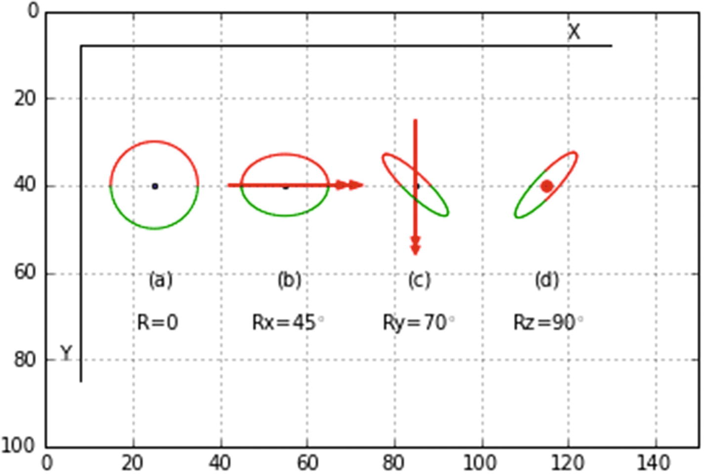
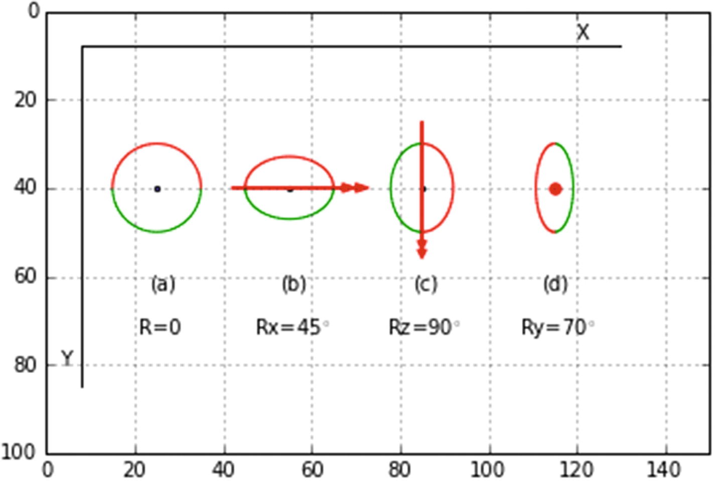
Sequential rotations of a circle created by Listing 3-3. Circle (a) is rotated by Rx=45° to (b), then by an additional rotation of Ry=70° to (c), and then by an additional rotation of Rz=90° to (d). Red indicates the upper half of circle. x and y axes show direction only, not coordinate values, which are indicated by the grid.
Listing 3-3 is similar to the preceding modified version of Listings 3-1 and 3-2 where you did sequential rotations of a box. In that program, the box had eight corners, which had to be transformed and updated with every rotation. Here you have a circle, which has many more points, to transform and update.
In lines 23-38, you fill lists between lines 33 and 38 with starting values of local and global coordinates of points around the circumference of the circle. They are spaced dphi=5° apart as shown in line 25. The circle’s radius is 10 as shown in line 27. The empty lists were previously defined in lines 14-20. As the loop starting at line 29 advances around the circle with angle phi, lines 30 to 32 calculate the local coordinates of each point. Lines 33-38 add the coordinates to the list using the append() function, which adds elements to a list. For example, with each cycle through the loop line 33 appends (adds) the local value of xp at the current angle phi to the x list. Since you are just filling the list at this point, you can use xp,yp,zp to also fill the xg, yg, and zg lists in lines 36-38. Note that zp=0 (program line 32) in this initial definition of the circle. That is, the circle starts off flat in the x,y plane. Subsequent rotations will be around that initial orientation.
Lines 41-72 define the transformation functions as before. The circle plotting function extends from line 75-86. Lines are used to plot the circle. The plotting loop runs from 78-82. Line 86 plots a dot at the center.
Rather than counting the number of points around the circle, you use the range(len(x)) function to give the number of elements in the lists. You can use the length of x as a measure since all lists have the same length. Lines 79-82 plot the top half red and the bottom half green. Lines 83-84 update the last xg any yg global coordinates to use when plotting the lines as before. You don’t need to include zg here since you use only xg and yg when plotting. Lines 89-108 transform coordinates as was done in Listings 3-1 and 3-2. The difference is here you have to deal with lists len(x) long whereas previously you had only eight corners.
Program SEQUENTIALCIRCLES
3.8 Matrix Concatenation
Circle (a) is rotated sequentially by Rx=45° to (b), then by an additional rotation of Rz=90° to (c), followed by an additional rotation of Ry=70 to (d). Red indicates the lower half of circle. x and y axes show direction only, not coordinate values, which are indicated by the grid.
You can demonstrate this yourself. Take a book and place it on the edge of your desk front side up, top facing to the right. Imagine the desk’s edge is the x direction going from left to right. Next, rotate it 90 degrees around the x direction, followed by 90 degrees around the z direction. This is RxRz. The book will be upside down with the front facing you. Then reverse the order by rotating around the z direction first followed by the x direction. This is RzRx. As you can see, you get a different final orientation of the book in the two cases.
![$$ left[{P}^{prime}
ight]=left[ Rz
ight]kern0.1em left[ Rx
ight]kern0.1em left[P
ight] $$](http://images-20200215.ebookreading.net/10/3/3/9781484233788/9781484233788__python-graphics-a__9781484233788__images__456962_1_En_3_Chapter__456962_1_En_3_Chapter_TeX_Equ64.png)
![$$ left[{P}^{prime}
ight]=left[ Rx
ight]kern0.1em left[ Rz
ight]kern0.1em left[P
ight] $$](http://images-20200215.ebookreading.net/10/3/3/9781484233788/9781484233788__python-graphics-a__9781484233788__images__456962_1_En_3_Chapter__456962_1_En_3_Chapter_TeX_Equ65.png)
![$$ left[ Rx
ight]kern0.1em left[ Rz
ight]
e left[ Rz
ight]kern0.1em left[ Rx
ight] $$](http://images-20200215.ebookreading.net/10/3/3/9781484233788/9781484233788__python-graphics-a__9781484233788__images__456962_1_En_3_Chapter__456962_1_En_3_Chapter_TeX_Equ66.png)


Each of these combinations involves three separate rotations. You could multiply the three transformation matrices shown in Equations 3-55, 3-56, and 3-57 to get a single transformation matrix for each of these combinations. You could then write a program that would execute each of these combinations: select one combination, input the three angles, and then get the final rotation. But what if you wanted more than three rotations, such as RyRzRxRyRz? That would require a lot of matrix multiplying! Clearly it’s much easier to incorporate the sequencing by coding it into the Python program and updating coordinates after each transformation, as you have learned how to do here.
To produce Figure 3-12, lines 110-136 of Listing 3-3 were replaced with the code in Listing 3-4.
Program SEQUENTIALCIRCLESUPDATE
Here you have performed the operation RxRzRy, reversing the order of the last two transformations. Circle (a) is plotted as before with Rx=0 in line 111. Also as before, circle (b) is plotted next with Rx=45 degrees in line 118. The difference is in lines 124-136 where the rotations Ry and Rz are reversed and Rz is plotted before Ry. The angles have the same values as before. Rearranging the order of plotting is easy; just cut and paste sections of the code. But be sure to update the center coordinates xc, yc, and zc. You could make the program a lot more user-friendly by introducing the input() function, which will give you the ability to input the order of transformations through the keyboard. You could then enter the rotations Rx,Ry, or Rz and the amount and the center coordinates in any order. You will do that next.
3.9 Keyboard Data Entry with Functional Program Structure
As you saw in the discussion of matrix concatenation, rearranging the order of rotations in a program can be a useful option. However, as you will see in this section, entering data via the keyboard is much more satisfactory. You will also use a functional programming structure where a few lines of code control various predefined functions that carry out the various operations. This will give you great flexibility in controlling the program.
Listing 3-5 produced the results shown in Figures 3-13 through 3-16. The first figure shows a circle rotated around the x direction by 0°; the second around the y direction by 60°; the third around the x direction by 45°; and the fourth around the z direction by 90°. All rotations are added to the previous orientation of the circle. The axis of rotation and the amount were entered through the keyboard. The sequence of rotation directions did not matter, nor did the number of rotations.
Referring to Listing 3-5, lines 111-113 specify the circle’s center coordinates. All circles have the same center coordinates. The while True: statement in line 115 keeps the data entry loop running so you can do an unlimited number of sequential rotations. Line 116 asks you to specify the axis of rotation in the Spyder output pane. Enter x,y, or z in lower case letters. To exit the loop, press the Enter key. (Important: If you are using the Spyder console, be sure to click the mouse with the cursor in the output pane before entering anything. If you forget and leave it in the program pane, you are liable to get an unwanted x,y, or z imbedded somewhere in the program. If this happens, go to the top of the screen and open a new console. This essentially starts the program over.). If you enter x (lower case), line 118 asks for the angle of rotation Rx. Enter it as a positive or negative angle in degrees. The input() function returns a string. The float command converts it to a float. Line 119 then invokes function plotcirclex(), which plots the rotated circle. Ry and Rz rotations are carried out in a similar way. Note there is no restriction on the sequence or the number of rotations. Line 126 checks to see if you entered a blank for axis, in which case line 127 exits the program. All circles are rotated around the same center, xc,yc,zc. If you want to be able to move the centers of each circle, just add input() lines for the center coordinates between lines 115 and 116.
Lines 89-108 rotate and update the coordinates of the circle’s circumferential points as was done in Listing 3-3. In function plotcircle() , lines 71-86 do the plotting. Each time this function is invoked, the axes and grid are replotted. Line 86 shows the latest plot.
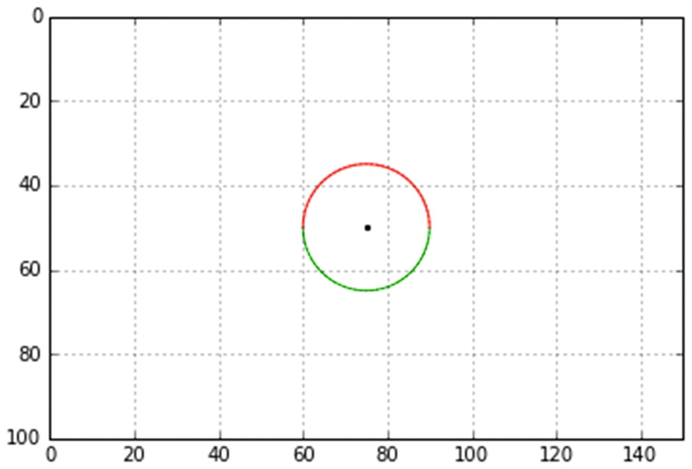
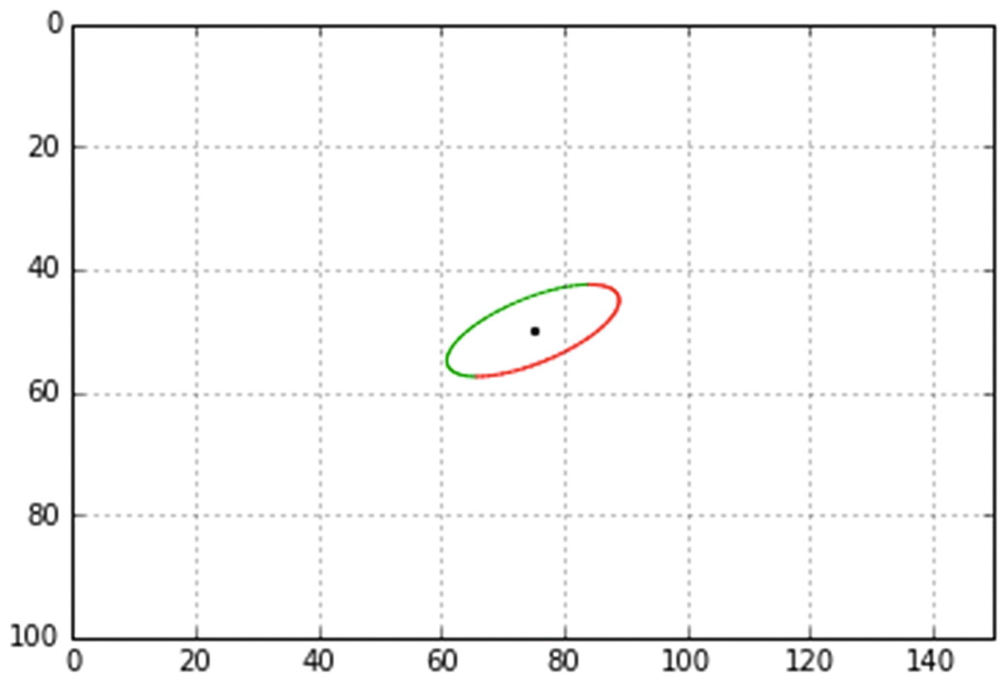
The circle is rotated around the x axis by 0°
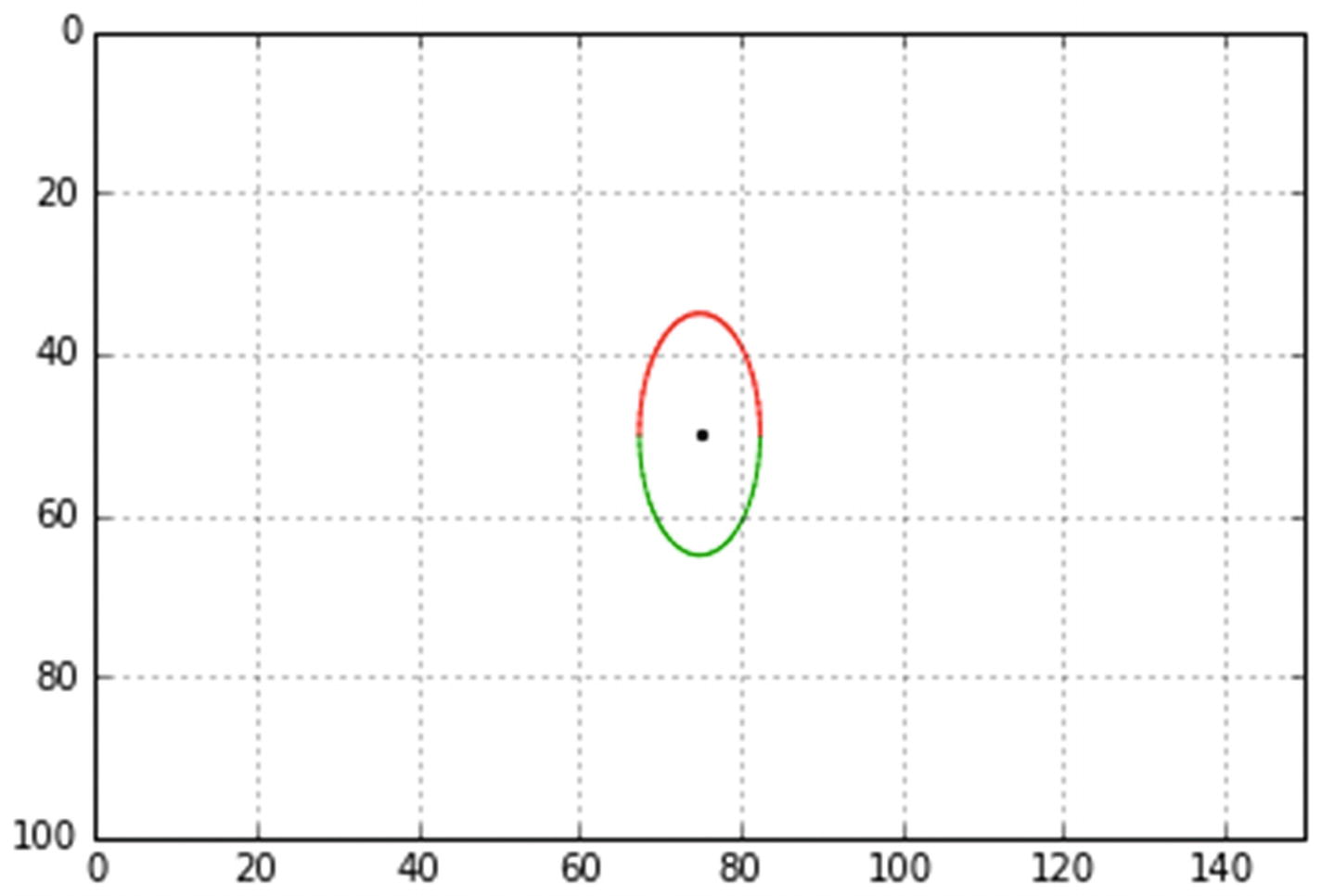
The previous circle is rotated around the y axis by 60°
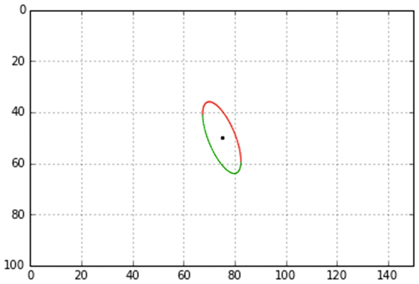
The previous circle is rotated around the y axis by 45°
The previous circle is rotated around the z axis by 90°
Program KEYBOARDDATAENTRY
3.10 Summary
In this chapter, you learned how to construct three-dimensional coordinate axes and three-dimensional shapes and rotate them around the three coordinate directions. This involved derivation of rotation transformations around the three coordinate directions. You saw the difference between rotating an object once from its original orientation and rotating it in sequential steps where each subsequent rotation uses the object’s coordinates from the prior rotation as the starting point. You explored the idea that the sequence of rotations is important; Rx,Ry,Rz does not produce the same results as Rx,Rz,Ry. This was shown by matrix concatenation. Finally, you developed a program where sequential rotations could be entered through the keyboard as opposed to specifying them in the program. All of this work involved the use of lists.