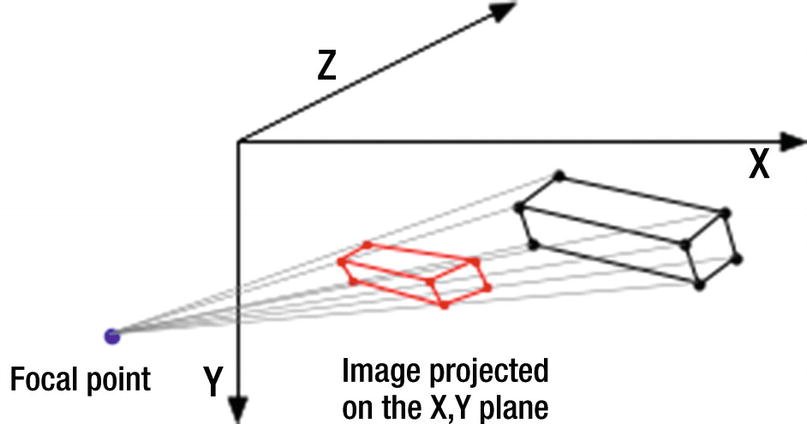
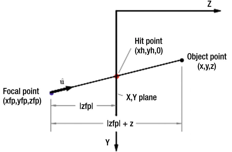
Geometry used to project a perspective image of an object on the x,y plane
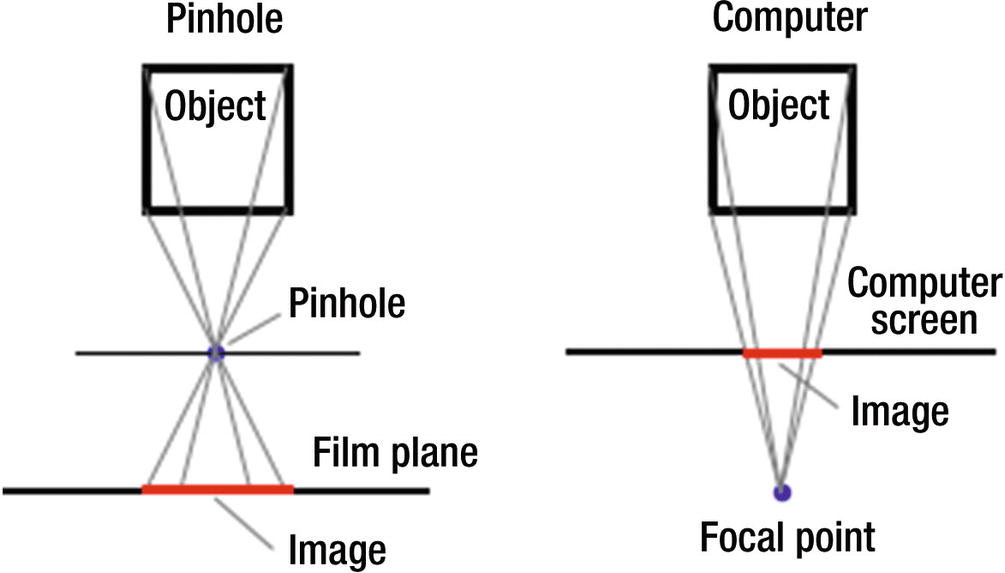
Pinhole camera vs. computer projection geometry
Figures 4-3 and 4-4 show the geometry you will use to construct your transformation. Figure 4-3 shows a three-dimensional object inside the x,y,z space. The focal point is outside the space at global coordinates (xfp,yfp,zfp). It can be anywhere in front of (-z direction) the x,y plane. Different locations will produce different views of the object, much as a camera will produce different images when photographing an object from different locations.
Imaginary rays emanating from the corners of the box pass through the x,y plane, which you can imagine is your computer screen. Each ray hits the x,y plane at a hit point (xh,yh,zh=0) on its way to the focal point of zh=0 since the x,y plane is at z=0. Connecting the hit points produced by the rays coming from the points comprising the object will produce a perspective image.


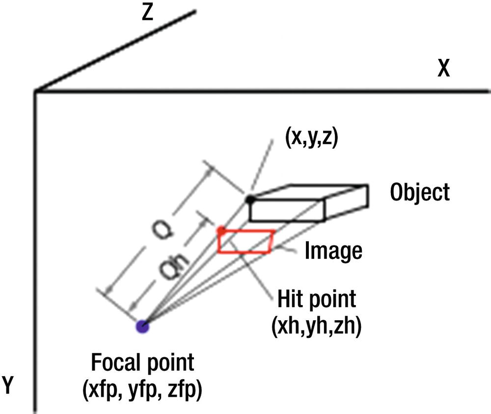
Perspective image projection geometry
Perspective image projection geometry side view
Listing 4-1 illustrates the use of the above model. It enables you to construct an object, rotate it, and then view it in perspective. The object, in this case a house, is defined in lines 14-29. Lines 14-16 establish corner coordinates x,y,z in local coordinates; that is, in relation to a point xc,yc,zc, which is set in lines 18-20. This is at the center of the house and it will be the center of rotation. Lines 22-29 convert x,y,z to global coordinates xg,yg,zg by adding elements to the empty lists set in lines 22-24. Lines 31-47 plot the house by connecting the corner points with lines.
Lines 50-63 define a function that rotates the local coordinates about xc,yc,zc, saving the results as xg,yg,zg. It uses function roty, which is defined in lines 54-63. This function was used in prior programs. It is the only rotation function in this program, which means you can only rotate around the y direction. Next is the perspective transformation perspective(xfp,yfp,zfp); it implements Equations 4-1 through 4-12, developed above. The loop beginning in line 67 calculates the coordinates of the hit point for rays that go to the focal point from each of the object’s corner points. The hit points, in terms of global coordinates, are saved in lines 79-81.
Control of the program takes place in lines 83-95. Lines 83-85 define the location of the focal point; lines 87-89 the house’s center point. Ry in line 91 specifies the angle of rotation about the y direction. Line 93 then invokes function plothouse(xc,yc,zc,Ry), which rotates the house. Line 94 invokes perspective(xfp,yfp,zfp), which performs the perspective transformation. Line 95 plots the house. This could have been incorporated in the function perspective but it has been placed here to illustrate the sequence of operations.
Program PERSPECTIVE
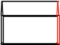
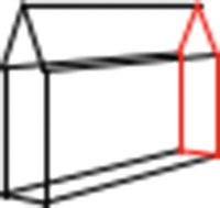
Perspective image with Ry=0, zfp=-100
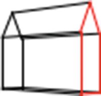
Perspective image with Ry=45, zfp=-100
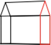
Perspective image with Ry=45, zfp=-600
Perspective image with Ry=-60, zfp=-100, xc=40, yc=70, xfp=100, zfp=-80
The question is, where to place the focal point. If you’re projecting the image onto the x,y plane, clearly it should be in front of that plane (i.e. i the -z direction). But what about the x,y coordinates of the focal point? The best results, most like what would be seen by the human eye, would be to place it at the same x,y coordinates as the house’s center. Of course, if there are many objects in the model, such as more houses and trees, it is not obvious where to place the focal point. The best results will be obtained by situating it in front of the x,y plane at the coordinates that correspond to the approximate center of the model. This is akin to aiming a camera at the center of a scene to be photographed. The painter Vermeer chose this structure in many of his paintings. In fact, in some of his canvases art historians have found a nail hole at the vanishing point where all parallel lines such as room corners and floor tiles converge. The nail hole is in the approximate center of the scene. It is believed he tied a string to a nail and used it to trace the converging lines, much as you have used lines in your algorithm. You can see this structure in many of Vermeer’s interior paintings.
4.1 Summary
In this chapter, you learned how to construct a perspective view. The geometry is based on the simple box camera. You had the perspective image projected onto the x,y plane. You could have used any of the other coordinate planes, for example the x,z plane; the geometry would be similar. You explored the question of where to place the focal point, which corresponds to the observation point of a viewer or a camera. The answer is, unless you are looking for an unusual image, at the approximate center of the model. This was the structure used by Vermeer in many of his paintings.