4
Writing Your First Amazon Braket Code Sample
In this chapter, we will go over some very basic code to get started in Amazon Braket. We will create a very simple quantum circuit to represent a binary number on a quantum register. This will demonstrate the basics of how to set up a quantum circuit and then measure it on a quantum device. We will spend some time understanding how to access the devices through the code and estimating the cost of running a quantum circuit on a device. Then, we will create the quantum circuit and run it. Finally, we can get a more accurate picture of the cost of execution. In this chapter, we will only use two simple quantum gates; however, we will use them somewhat classically, so a deep explanation of the complex nature of quantum states and gate operations will not be needed.
In this chapter, we will cover the following key topics:
- Finding active devices
- Assigning a device
- Cost estimation
- Creating a simple quantum circuit
- Running a circuit on a simulator device
- Actual simulator costs
Technical requirements
The source code for this chapter can be found in the following GitHub repository:
Finding active devices
In the previous chapters, we discussed the devices that are available in Amazon Braket. Here, we will look at how to access the device information through code. This will become necessary as new devices are added.
Note: Amazon Braket Device Availability
Carefully evaluate the devices present when you purchase this book and run this code. New devices might have been added, and some devices might have been turned off. Also, depending on the region in which you set up your config file, you might see different devices. Since D-Wave is not available through Amaon Braket, we will do a short test to ensure the direct method to D-Wave LEAP is working at the end of the refreshed code provided online with this chapter.
To do this, perform the following steps:
- The following code retrieves active devices in Amazon Braket in the form of a list. The following output has been formatted to be easier to read:
from braket.aws import AwsDevice
device_list=AwsDevice.get_devices(statuses=['ONLINE'])
print(device_list)
Output:
[Device('name': Advantage_system4.1, 'arn': arn:aws:braket:::device/qpu/d-wave/Advantage_system4),
Device('name': Advantage_system6.1, 'arn': arn:aws:braket:us-west-2::device/qpu/d-wave/Advantage_system6),
Device('name': Aspen-M-1, 'arn': arn:aws:braket:us-west-1::device/qpu/rigetti/Aspen-M-1),
Device('name': DW_2000Q_6, 'arn': arn:aws:braket:::device/qpu/d-wave/DW_2000Q_6),
Device('name': IonQ Device, 'arn': arn:aws:braket:::device/qpu/ionq/ionQdevice),
Device('name': SV1, 'arn': arn:aws:braket:::device/quantum-simulator/amazon/sv1),
Device('name': TN1, 'arn': arn:aws:braket:::device/quantum-simulator/amazon/tn1),
Device('name': dm1, 'arn': arn:aws:braket:::device/quantum-simulator/amazon/dm1)]
The device name and Amazon Resource Name (ARN) are returned. This long string contains information about whether the device is a QPU or a simulator, along with the device manufacturer and the QPU name.
- We can simply store the device names in a list so that we can assign a device with the name. The names are case sensitive:
device_name_list=[]
for device in device_list:
    device_name_list.append(device.name)
print('Valid device names: ',device_name_list)
Output:
Valid device names:  ['Advantage_system4.1', 'Advantage_
system6.1', 'Aspen-M-1', 'DW_2000Q_6', 'IonQ Device', 'SV1',
'TN1', 'dm1']]
- A helpful function that can be used to quickly get the list of available devices is as follows:
def available_devices(): from braket.aws import AwsDevice device_list=AwsDevice.get_devices(statuses=['ONLINE']) device_name_list=[] for device in device_list: device_name_list.append(device.name) #print('Valid device names: ',device_name_list) return(device_name_list) - Once the function has been executed, we should get the names of all the available devices:
available_devices()
Output:
['Advantage_system4.1',
 'Advantage_system6.1',
 'Aspen-M-1',
 'DW_2000Q_6',
 'IonQ Device',
 'SV1',
 'TN1',
 'dm1']
Since the devices are regularly upgraded, please run this function and make appropriate changes as you progress through this book. In the next section, we can use this information to assign a device that you want to work with.
Assigning a device
We can assign various devices available in Amazon Braket, however, each device uses different resources. The local simulator uses the local computer resources to execute the circuit if using a remote connection.The Amazon Braket simulators TN1 and SV1 use Amazon resources. External quantum devices such those available from D-Wave, IonQ, or Rigetti use compute time on the quantum hardware housed at the respective facilities of these providers in Barnaby, Maryland, or California respectively.
Each type of device has a limit in terms of the number of qubits, the amount of circuit information it can handle, and in some cases, the depth of the circuit that it can execute. The circuit depth can be thought of as the number of columns of gate after the circuit has been converted into its low-level transpiled version. This is the version where all the gates on each qubit are packed together, as much as is feasible, using native gate operations on the hardware. Native gate operations are the basic gates that the gate-based quantum computer can execute on its Quantum Processing Unit (QPU). Other more complex gate operations are converted or transpiled into these native gates.
Using the local simulator
Before a circuit can be executed on a device, we need to assign the device. First, let’s see how to assign the local simulator. The local simulator can handle up to 25 qubits without noise, or up to 12 qubits with noise, and its execution will depend upon the memory and filesystem limitations of the computer it is run on.
The local simulator (without noise) is assigned using either of the following functions. The first is as follows:
device = LocalSimulator()
Alternatively, you can use the following:
device = LocalSimulator(backend="braket_sv")
The localSimulator() function uses the Braket state vector simulator. Since quantum computing produces probabilistic answers, the state vector simulator calculates all the exact probabilities of the final state. The actual values produced in the final measured results reflect these probabilities, and the accuracy of this increases with the number of shots. For example, if we know that the probability of getting each side of dice is 1/6, then as we increase the number of times we roll a dice, the more accurately the results will reflect this probability.
Using Amazon simulators or quantum devices
We will now assign Amazon simulators or external quantum devices for use. Here is an example of how to assign a device using the arn value:
- This is the typical way of assigning a device for use:
rigetti = AwsDevice("arn:aws:braket:us-west-1::device/qpu/rigetti/Aspen-M-1") print(rigetti)
Output:
Device('name': Aspen-M-1, 'arn': arn:aws:braket:us-west-1::device/qpu/rigetti/Aspen-M-1)- Rather than providing the full arn value, the following function only requires the device name to set the device. Here, Name refers to the device name as returned by the available_devices() function:
device=AwsDevice.get_devices(names=Name)
For example, if you're using the SV1 device, it will be as follows:
sv1=AwsDevice.get_devices(names='SV1')
print(sv1)
Output:
[Device('name': SV1, 'arn': arn:aws:braket:::device/quantum-simulator/amazon/sv1)]Note: Device Name
The device name is case-sensitive.
- The set_device(Name) function can be helpful as a reusable function to set the device, based on the name. In this case, the full arn value is not necessary:
def set_device(Name): device_list=AwsDevice.get_devices(names=Name) if len(device_list)==1: device=device_list[0] print(device) return(device) else: print('No device found') print('use name from list', available_devices()) - In the case of a wrong name, an error message with available device names will be given:
device=set_device('svi')
Output:
No device found
use name from list ['Advantage_system1.1', 'Aspen-9', 'DW_2000Q_6', 'IonQ Device', 'SV1', 'TN1', 'dm1']
Now that we know various ways and options in which to assign a device in Amazon Braket, in the next section, let’s find the cost of the device.
Estimating the cost of the device
The following code shows how to estimate the cost of the different devices. Because we assigned the device in the last section, we can further use the device to determine the cost. The estimate_cost function has the appropriate calculations to estimate the cost of the device that is passed through along with the number of shots. The default number of shots is 1000.
Let’s get started! Perform the following steps:
- The following function calculates the costs of the simulators on a cost per minute basis, while the cost of the quantum devices is calculated based on the QPU rate and the number of shots. Note that this function is making some assumptions about the cost_per_task amount, and the available QPUs and simulators. Please update these in the code if cost_per_task has changed in the Amazon Braket pricing table:
def estimate_cost(device,num_shots=1000):
    #device=set_device(Name)
    cost_per_task=0.30
    Name=device.name
    if Name in ['SV1','TN1','dm1']:
        price_per_min=
          device.properties.service.deviceCost.price
        unit=device.properties.service.deviceCost.unit
        print('simulator cost per ',unit,': $',
               price_per_min)
        print('total cost cannot be estimated')
    elif Name in['Advantage_system6.1',
      'Advantage_system4.1','DW_2000Q_6',
      'Aspen-M-1','IonQ Device']:
        price_per_shot=
          device.properties.service.deviceCost.price
        unit=device.properties.service.deviceCost.unit
        print('device cost per ',unit,': $',
               price_per_shot)
        print('total cost for {} shots is
              ${:.2f}'.format(num_shots,
              cost_per_task+num_shots*price_per_shot))
    else:
        print('device not found')
        print('use name from list',
               available_devices())
We use the preceding function with the SV1 device. Since the cost of the SV1 device is based on the time of execution, it is not possible to estimate the actual cost prior to execution. We will see how to calculate the actual costs after execution later in this chapter.
- The next line of code shows the result of adding SV1, a simulator, to the estimate_cost function:
device_name='SV1'
device=set_device(device_name)
estimate_cost(device)
Output:
Device('name': SV1, 'arn': arn:aws:braket:::device/quantum-simulator/amazon/sv1)
simulator cost per  minute : $ 0.075
total cost cannot be estimated
Since we picked a simulator, the device cost is dependent on the execution time, so this cannot be accurately calculated. Please try using different device names to see what results you get for the simulators versus the QPUs.
The following function can help you to more accurately estimate the cost based on the number of measured qubits. For this equation, we will use a heuristic that, for each possible state in the output of our quantum device, we should measure at least 25 times. The number of possible states in the output is 2n, where n is the number of measured qubits.

This provides the minimum number of shots based on the number of qubits that are being measured. You can update this equation, as desired, according to your own preference.
- As the number of qubits increases, each device reaches its maximum number of shots limit. If the number of recommended shots is greater than the maximum number of shots of the device, the maximum number of shots is returned by the following function:
def estimate_cost_measured_qubits(device,measured_qubits): #device=set_device(Name) min_shots_per_variable=25 max_shots=device.properties.service.shotsRange[1] print('max shots:', max_shots) num_shots= min_shots_per_variable*2**measured_qubits if num_shots>max_shots: num_shots=max_shots print('for {} measured qubits the maximum allowed shots: {:,}'.format( measured_qubits,num_shots)) else: print('for {} measured qubits the number of shots recommended: {:,}'.format( measured_qubits,num_shots)) estimate_cost(device,num_shots) - For example, let’s determine the cost of using IonQ with a circuit where we will measure 5 qubits:
device=set_device('IonQ Device')
estimate_cost_measured_qubits(device, 5)
Output:
Device('name': IonQ Device, 'arn': arn:aws:braket:::device/qpu/ionq/ionQdevice)
max shots: 10000
for 5 measured qubits the number of shots recommended: 800
device cost per  shot : $ 0.01
total cost for 800 shots is $8.30- The next block includes the code to give the cost estimate for each of the devices based on the maximum number of allowed shots and the maximum number of qubits. Therefore, for now, in the case of the Rigetti and IonQ devices, the maximum number of qubits has been hardcoded in this function. When you create your circuit, the number you should use is the actual number of qubits you are using. Also, keep in mind the simulators do not give a cost upfront, as the cost is estimate at the end of the execution based on the time to solution. Now, let’s look at each of the three categories of devices separately:
Output:
Device('name': SV1, 'arn': arn:aws:braket:::device/quantum-simulator/amazon/sv1)
max shots: 100000
for 34 measured qubits the maximum allowed shots: 100,000
simulator cost per  minute : $ 0.075
total cost cannot be estimated
---
Device('name': TN1, 'arn': arn:aws:braket:::device/quantum-simulator/amazon/tn1)
max shots: 1000
for 50 measured qubits the maximum allowed shots: 1,000
simulator cost per  minute : $ 0.275
total cost cannot be estimated
---
Device('name': dm1, 'arn': arn:aws:braket:::device/quantum-simulator/amazon/dm1)
max shots: 100000
for 17 measured qubits the maximum allowed shots: 100,000
simulator cost per  minute : $ 0.075
total cost cannot be estimated
---- The costs for the Rigetti and IonQ devices can be found using the following code:
for Name in ['Aspen-9','IonQ Device']:
    device=set_device(Name)
    if Name=='Aspen-9':
        qubit_count=31
    elif Name=='IonQ Device':
        qubit_count=11
    estimate_cost_measured_qubits(device, qubit_count)
    print('---')
Output:
Device('name': Aspen-M-1, 'arn': arn:aws:braket:us-west-1::device/qpu/rigetti/Aspen-M-1)
max shots: 100000
for 2048 measured qubits the maximum allowed shots: 100,000
device cost per  shot : $ 0.00035
total cost for 100000 shots is $35.30
---
Device('name': IonQ Device, 'arn': arn:aws:braket:::device/qpu/ionq/ionQdevice)
max shots: 10000
for 11 measured qubits the maximum allowed shots: 10,000
device cost per  shot : $ 0.01
total cost for 10000 shots is $100.30
As you can see, the device costs vary considerably. However, you can modify this function for your own needs and execute it prior to running a quantum circuit on a device based on the number of shots and the number of qubits measured.
- Since we could not estimate the cost of the simulators in advance, it is possible to calculate the cost after execution with the help of the following method, which returns the duration of the execution:
results.additional_metadata.simulatorMetadata.executionDuration
In this case, we would execute the quantum circuit on the device and then multiply the result of the preceding method by the cost per minute.
You have now experimented with some simple Braket functions to find the device name, assign a device and estimate its costs. In the case of simulators, we could not estimate the cost in advance, so we will come back to this after we have created a simple circuit and visualized that circuit in the following section.
In the next section, we will create a simple quantum circuit and execute it on a quantum simulator.
Creating a simple quantum circuit
Now we are ready to create a simple quantum circuit in Amazon Braket.
When creating a quantum circuit in Braket, it should be noted that the circuit expands as different qubits are identified. Figure 4.1 shows the quantum circuit we are creating:

Figure 4.1 – Visualizing a simple circuit in Amazon Braket
The circuit starts with a state of |0⟩ on each qubit. In this chapter, please do not worry about the | and the ⟩ brakets around the numbers. We will review this later in Chapter 6, Using Gate-Based Quantum Computers - Qubits and Quantum Circuits. We will only use two very simple quantum gates. For our purposes right now, the X gate will also refer to as a NOT gate. The X gate will change the |0⟩ state into a |1⟩ state and vice versa. Additionally, we will use the identity gate, I, which leaves the original |0⟩ value as is. If the |1⟩ state was preceded by the identity gate, I, then that value would not change either.
For now, we will treat the circuit as dealing with classical values only. Therefore, we will use 0 for the |0⟩ state and 1 for the |1⟩ state.
In the following code, we will start by loading the appropriate Amazon Braket libraries along with matplotlib:
from braket.circuits import Circuit, Gate, Observable
from braket.devices import LocalSimulator
from braket.aws import AwsDevice
import matplotlib.pyplot as plt
%matplotlib inline
Now, we can begin the creation of our first quantum circuit by using the Circuit()function. In the following example, bits is assigned a quantum circuit with the identity gate I on qubit 0 and the X gate on qubit 1:
bits = Circuit().i(0).x(1)
print(bits)
Output:
T : |0|
q0 : -I-
q1 : -X-
T : |0|
This simple quantum circuit can be read as having started with the 00 register and, after running through the two gates, I and X, together, results in the register containing a value of 01:
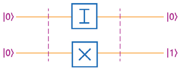
Figure 4.2 – A simple circuit using the I and X gates to produce 01
We have created a very basic quantum circuit. Now, we can implement this for any number, N, in the next section.
Putting together a simple quantum circuit example
Below is the full code that is needed to assign the local simulator device and then run the bits circuit on the local simulator device with 1,000 shots.
The results are returned to the counts variable. The results are printed and then plotted:
device = LocalSimulator()
result = device.run(bits, shots=1000).result()
counts = result.measurement_counts
print(counts)
plt.bar(counts.keys(), counts.values());
plt.xlabel('states');
plt.ylabel('counts');Output:
Counter({'01': 1000})The following diagram shows the histogram plot of the probabilities of the results:

Figure 4.3 – Results showing 01 as the only resulting state; all 1,000 shots have the same answer
The results are probabilistic. However, since we only converted 00 into 01, the results are always 01. This is the only state that is produced on this simulator since the |01⟩ state has a 100% probability of being in the answer.
Representing a binary value using a quantum circuit
Now we can create a simple function that takes a decimal number and converts it into a quantum state that represents the binary value of the number.
In the following function, first, we get the binary value of the number and then create a quantum circuit that has the same number of qubits as the length of the binary value representing the number. Next, we represent the binary number as a quantum state. In the case of a zero in the binary number we will place the I gate and for a one in the binary number we will place the X gate. Please note that the X gate will convert the original state of |0⟩ into a |1⟩ state and the I gate does not change the state so leaves the original state of |0⟩ as is. Let us now review the code:
def build_binary_circ(N):
    binary_num=bin(N)[2:]
    num_qubits=len(binary_num)
    print(binary_num)
    binary_circuit=Circuit()
    position=0
    for bit in binary_num:
        #print(bit)
        if bit=='0':
            binary_circuit.i(position)
        else:
            binary_circuit.x(position)
        position+=1
    return(binary_circuit)
Now we can run the function. In the following example, we use the number 6, which has been converted into the binary value of 110. The function is then used to put an X gate on qubit 0, an X gate on qubit 1, and an I identity gate on qubit 2:
binary_circuit=build_binary_circ(6)
print(binary_circuit)
Output:
110
T : |0|
q0 : -X-
q1 : -X-
q2 : -I-
T : |0|
The preceding output is a representation of the quantum circuit.
Next, we use LocalSimulator() function as the device and run the circuit generated by the build_binary_circ() function:
device = LocalSimulator()
result = device.run(binary_circuit, shots=1000).result()
counts = result.measurement_counts
print(counts)
Output:
Counter({'110': 1000})Again, the output is based on the probabilities, which are 100% for the one answer of 110. We get the correct value, which is the binary representation of 6.
Now we will plot the bar chart to show the same result within a plot:
plt.bar(counts.keys(), counts.values());
plt.xlabel('states');
plt.ylabel('counts');
As expected, the following plot only has one value of 110 represented for all 1,000 results:
Figure 4.4 – Results showing 110 encoded in the quantum circuit
We have created a simple quantum circuit and executed it on the local simulator. In the next section, we will take this one step further by executing the same circuit on an Amazon Braket simulator.
Running a circuit on the Amazon simulator
Now we have a circuit that we can run on a simulator. However, before we can run on the simulator device, we need to set the Amazon S3 bucket information. This will tell Braket where to save the resulting json output file. Then, we will create a simple function that will run the circuit on the desired device and plot the results. If you are interested in using the Amazon Braket console to check that your task has appeared in the task list, and also find the resulting output file in your S3 folder, please review Chapter 3, User Setup, Tasks, and Understanding Device Costs.
Let’s get started! Perform the following steps:
- First, you will have to use your appropriate Amazon Braket S3 bucket name along with the folder where the results should be stored. Remember to replace the values in the appropriate places in the following code:
# Enter the S3 bucket you created during onboarding in the code below
my_bucket = "amazon-braket-[your bucket]" # the name of the bucket
my_prefix = "[your folder]" # the name of the folder in the bucket
s3_folder = (my_bucket, my_prefix)
- Now, let’s create a run_circuit() function that will take device, circuit, shots, and s3_folder, execute the circuit on the device, and return the results:
def run_circuit(device, circuit, shots, s3_folder): import matplotlib.pyplot as plt %matplotlib inline result = device.run(binary_circuit, shots=shots, s3_destination_folder=s3_folder).result() counts = result.measurement_counts print(counts) plt.bar(counts.keys(), counts.values()); plt.xlabel('states'); plt.ylabel('counts'); return(result) - The next function is used to determine the actual simulator cost. This takes the actual time of execution of the circuit and calculates the cost based on the rate:
def actual_simulator_cost(device, result): price_per_min= device.properties.service.deviceCost.price price_per_ms=price_per_min/60/1000 unit=device.properties.service.deviceCost.unit duration_ms=result.additional_metadata .simulatorMetadata.executionDuration if unit=='minute': print('simulator cost per ',unit,': $', price_per_min) print('total execution time: ', duration_ms, "ms") print('total cost estimated: $',duration_ms*price_per_ms) - Now we are ready to execute the three functions that we have created. Let’s use the build_binary_circ() function to build a circuit that represents the number 2,896 in binary on a quantum register, run the circuit to evaluate the end state, and then get the cost for a sample run on SV1.
This first section creates the circuit to represent the binary number, as demonstrated earlier:
N=2896
qubit_count=len(bin(N))-2
print('qubit count: ', qubit_count)
binary_circuit=build_binary_circ(N)
print(binary_circuit)Output:
qubit count:  12
101101010000
T   : |0|
q0  : -X-
q1  : -I-
q2  : -X-
q3  : -X-
q4  : -I-
q5  : -X-
q6  : -I-
q7  : -X-
q8  : -I-
q9  : -I-
q10 : -I-
q11 : -I-
T   : |0|
- Now we can set the device to the Amazon Braket simulator, SV1. Then, we can run the cost estimation function that also shows the number of shots we should run based on the number of qubits measured.
We already know there is only one valid state in the result. Knowing this information, we can substantially reduce the number of shots on this simulator.
We use the estimate_cost_measured_qubits() function to estimate the cost for SV1:
device=set_device('SV1')
estimate_cost_measured_qubits(device, qubit_count)Output:
Device('name': SV1, 'arn': arn:aws:braket:::device/quantum-simulator/amazon/sv1)
max shots: 100000
for 12 measured qubits the maximum allowed shots: 100,000
simulator cost per  minute : $ 0.075
total cost cannot be estimated- In this case, and especially since we are using a simulator and understand there is only one valid state, we will only use 10 shots when we run the circuit. A new run_circuit() function is created to easily run a quantum circuit and plot the results.
Here is the code of the execution of the circuit, the raw results, and the resulting histogram. You can see that the same binary number is returned for all 10 shots:
result=run_circuit(device, binary_circuit, 10, s3_folder)
Output:
Counter({'101101010000': 10})

Figure 4.5 – Results showing 101101010000 encoded in the quantum circuit
Actual cost of using the Amazon simulator
Finally, we can get the actual cost of executing this circuit on the simulator by running the actual_simulator_cost() function:
actual_simulator_cost(device, result)
Output:
simulator cost per minute : $ 0.075
total execution time: 3 ms
total cost estimated: $ 3.7500000000000005e-06
Now, we have an accurate representation of the costs that will be incurred when we run a circuit on an Amazon Braket simulator.
Please refer to the updated online code provided with this chapter to run the sample code with D-Wave. The code creates a small matrix representing linear and quadratic weights on 3 qubits and gets back the minimum energy value.
Summary
In this chapter, we showed the basics of writing code in Amazon Braket by creating a simple quantum circuit, executing it on an Amazon Braket device, and displaying the probabilistic results.
We started by using the Amazon Braket functions to find the appropriate device and then got cost estimates for using that device based on the number of shots. Then, we created a simple circuit to display a binary number on a quantum register using the LocalSimulator() function. Finally, we ran that circuit on the SV1 simulator and got an accurate value for the cost of execution.
Further reading
In this chapter, we used a few functions to get the properties of the devices. The following two resources offer more details on how to determine other device properties and device capabilities:
- For more information on Amazon Braket Python Schemas, please visit https://amazon-braket-schemas-python.readthedocs.io/en/latest/index.html.
- For more information on the parameters that are used when calling devices, please visit https://amazon-braket-sdk-python.readthedocs.io/en/stable/_apidoc/braket.aws.aws_device.html.
- Detailed information on tracking pricing: https://docs.aws.amazon.com/braket/latest/developerguide/braket-pricing.html
- Detailed information on using D-Wave directly from D-Wave LEAP https://cloud.dwavesys.com/leap/resources
- Detailed information on how to use D-Wave through the AWS Marketplace https://aws.amazon.com/marketplace/seller-profile?id=aa4f61b5-7b1f-4984-9175-1a636281d694
- Detailed code example of using D-Wave through the AWS Marketplace https://aws.amazon.com/blogs/quantum-computing/using-d-wave-leap-from-the-aws-marketplace-with-amazon-braket-notebooks-and-braket-sdk/
Concluding Section 1
We now end Section 1. We have gone over the basics of Amazon Braket and its components.
In Chapter 1, Setting up Amazon Braket, we reviewed how to get started with Amazon Braket and its various components.
In Chapter 2, Braket Devices Explained, we looked at the devices that are available on Amazon Braket.
In Chapter 3, User Setup, Tasks, and Understanding Device Costs, we went into more detail about the user administration, including the user group setup and permissions, and we explained the cost structure of the devices.
In this chapter, we wrote a simple quantum circuit and executed it on the local and Amazon Braket SV1 simulators.
In Section 2, we will go over the mathematical and quantum concepts that are necessary to start using the quantum annealer, gate quantum computers, and hybrid circuits, which use both classical code and quantum computers. These building blocks and fundamentals will be necessary to gain an understanding of how quantum annealers are used and how quantum circuits are created. We will start by showing how D-Wave’s quantum annealer performs optimization using some simple use cases. Next we will start a journey towards doing the same using gate quantum computers. In Chapter 6, Using Gate-Based Quantum Computers - Qubits and Quantum Circuits, we will switch to understanding quantum gates based on linear algebra, and how those gates are used to create quantum circuits. We will then create simple quantum circuits and expand our understanding of circuits that represent Monte Carlo and then can be used to increase the probability of finding the global minimum of an objective function. This will lead us to developing the gate-based equivalent of an optimization algorithm which is called Quantum Approximate Optimization Alogrithm or QAOA. By Chapter 9, Running QAOA on Simulators and Amazon Braket Devices will try more elaborate use cases using this hybrid method and compare results with the D-Wave quantum annealer. This journey will require considerable patience as it includes a lot of details in how these algorithms are developed and considerable execution and experimentation to demonstrate the type of results returned by our current quantum computing devices and how to interpret and improve on those results.
This fundamental understanding of circuits will then be used when we solve real-world use cases in Section 3.
Let’s get started with the next section.